Section 1: Why Engineering Needs Physics-Informed Neural Networks
Why Data-Driven Machine Learning Struggles with Physical Systems
Traditional machine learning models learn relationships between inputs and outputs by identifying patterns in training data, making them useful for prediction tasks where sufficient representative observations are available. However, engineering systems often operate under physical constraints that a conventional neural network does not automatically understand, including conservation of mass, conservation of energy, momentum relationships, material behavior, and governing differential equations. A network trained only on measurements may produce predictions that fit the observed examples but violate these constraints in regions where data is sparse, particularly when the system operates under conditions that differ from those represented in the training dataset.
Consider a heat-transfer application in which engineers want to predict temperature throughout a component based on measurements collected from a limited number of sensors. A conventional neural network may learn the relationship between sensor readings and temperature values within the sampled operating conditions, but it may behave unpredictably in locations where no sensors are installed or when the component is exposed to a new heating pattern. Even if the model achieves low prediction error on the training and validation datasets, its predictions may not satisfy the governing heat equation or the boundary conditions imposed by the component's physical environment. This limitation becomes particularly important when engineers need reliable estimates across an entire spatial domain rather than predictions only at locations where measurements are available.
Collecting more experimental data can improve a data-driven model, but obtaining high-quality engineering measurements is often expensive, time-consuming, or constrained by safety and equipment limitations. Running laboratory experiments across a wide range of operating conditions may require specialized facilities, while instrumenting every region of a complex physical system may be impractical, leaving engineers with incomplete observations and significant uncertainty about the underlying physical behavior. Physics-informed neural networks address this problem by incorporating known physical relationships into the learning process, enabling the model to use both available data and the mathematical structure of the system rather than relying exclusively on patterns inferred from measurements.
How Physical Laws Provide Structure Beyond Historical Measurements
Physical systems are governed by relationships that describe how quantities change across space and time, and these relationships can provide valuable information even when experimental observations are limited. Differential equations describe how physical fields such as temperature, pressure, velocity, displacement, and concentration evolve, while boundary conditions specify how a system interacts with its surroundings and initial conditions establish its state at the beginning of a time-dependent problem. Conservation laws and constitutive relationships provide further constraints, allowing engineers to describe behavior such as energy transfer, fluid motion, and material deformation through equations that connect measurable quantities and their derivatives.
Physics-informed neural networks incorporate these relationships into model training by penalizing predictions that violate the governing equations or specified physical constraints. Rather than learning only from observed input-output pairs, a PINN can be trained to approximate a physical field while minimizing both the difference between predictions and available measurements and the residuals produced when the predicted field is substituted into the relevant differential equations. This approach gives the learning process an additional source of information about expected behavior, which can help constrain predictions in areas where direct measurements are unavailable, provided that the governing equations and boundary conditions adequately represent the physical system being modeled.
The role of physical knowledge becomes particularly important when a model must generalize beyond the exact conditions represented in the training data, since equation-based constraints can discourage some physically implausible solutions that a purely data-driven model might otherwise produce. For example, a PINN used to model heat diffusion can incorporate the heat equation together with the material properties and boundary conditions, encouraging the predicted temperature field to remain consistent with the mathematical description of the process. However, physical constraints do not automatically guarantee an accurate solution, because incorrect assumptions, uncertain material properties, poorly balanced loss functions, or optimization difficulties can still produce predictions that fit neither the observations nor the real system reliably.
How PINNs Relate to Numerical Simulation and Scientific Machine Learning
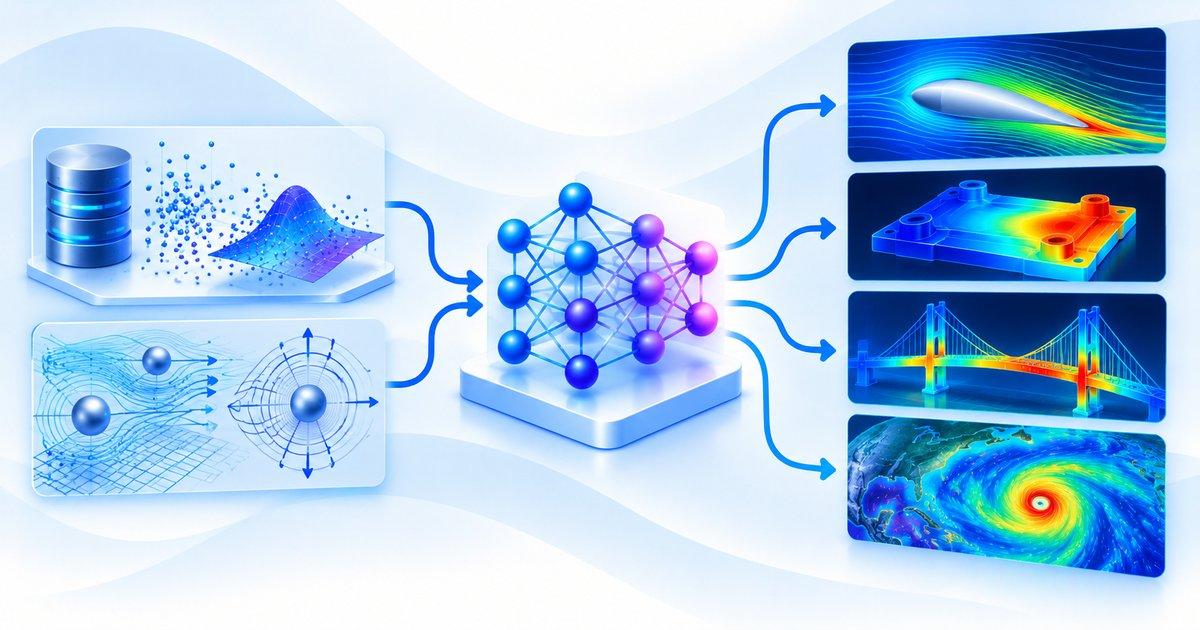
Physics-informed neural networks belong to the broader field of scientific machine learning, which combines data-driven techniques with scientific knowledge, physical equations, and computational methods to model complex systems. Conventional numerical solvers discretize governing equations using methods such as finite differences, finite elements, or finite volumes, then solve the resulting numerical problem over a defined spatial or temporal domain. PINNs take a different approach by representing the physical solution with a neural network and training its parameters to satisfy the governing equations and available observations, creating a continuous function that can be evaluated at selected points within the modeled domain.
This distinction can make PINNs attractive for certain problems, particularly when engineers want to combine sparse measurements with physical constraints, estimate unknown parameters, or develop a reusable approximation for repeated evaluations. However, a PINN is not simply a faster numerical solver, because training it can be computationally expensive and challenging, especially for stiff equations, complex geometries, sharp gradients, or systems with multiple spatial and temporal scales. Established numerical methods may remain more accurate, stable, and computationally efficient for many forward simulation tasks, making it important to choose the approach according to the problem's mathematical properties and engineering requirements rather than assuming that a neural network will outperform traditional simulation.
The relationship between scientific ML and engineering systems is also illustrated by “Machine Learning for Digital Twins: How AI Is Learning to Model the Physical World”, where machine learning supports the estimation and prediction of system behavior within a broader physical or operational context. PINNs can contribute to similar workflows by combining measured data with physical constraints, potentially supporting parameter estimation, approximate field reconstruction, or faster repeated evaluations after a suitable model has been trained and validated. Their practical value must nevertheless be assessed against trusted numerical solutions, experimental observations, computational cost, and the consequences of prediction error, since the most appropriate modeling approach depends on the specific engineering task and the reliability requirements of the application.
Key Takeaway
Physics-informed neural networks combine neural function approximation with governing equations, boundary conditions, initial conditions, and available experimental measurements to model physical systems under data constraints. They can support both forward simulation and inverse parameter estimation, particularly when engineers need to combine sparse observations with known physical relationships, but their effectiveness depends on the validity of the equations, the quality of the data, and the difficulty of the optimization problem. By evaluating PINNs against suitable numerical solvers and data-driven baselines, engineering teams can determine where physics-informed learning provides a practical benefit without assuming that it universally replaces established simulation methods.
Section 2: How Physics-Informed Neural Networks Incorporate Physical Laws
Representing Physical Fields and System States With Neural Networks
Physics-informed neural networks represent physical quantities as continuous functions of spatial coordinates, time, and relevant system parameters, allowing a neural network to approximate how a physical system behaves throughout a defined domain. Instead of learning only a mapping from measured inputs to observed outputs, a PINN can approximate fields such as temperature, pressure, velocity, displacement, or concentration using a function parameterized by neural network weights. For a heat-transfer problem, for example, the network may take spatial coordinates and time as inputs and predict the temperature at a particular location, producing a representation that can be evaluated at points where no experimental sensors are installed.
The network architecture should reflect the requirements of the physical problem, including the dimensionality of the domain, the smoothness of the expected solution, and whether the system changes over time. A steady-state problem may require only spatial coordinates as inputs, whereas a transient simulation needs both spatial and temporal information to represent changes in the physical field. Additional inputs can represent system parameters such as thermal conductivity, fluid viscosity, external forcing, or material properties, allowing a single network to approximate solutions across multiple operating conditions when the training strategy and architecture support that objective. These design decisions influence the model's capacity to represent the solution and its ability to generalize across the physical domain.
Unlike a conventional regression model trained exclusively to reproduce observed measurements, a PINN uses its neural representation as part of a larger optimization process that incorporates physical constraints. The predicted field can be differentiated with respect to its inputs, allowing the network to estimate the derivatives needed by governing differential equations, while the trainable parameters are adjusted to reduce discrepancies between the predicted solution and the required physical behavior. This enables the model to use both experimental observations and mathematical structure when learning a solution, although the quality of the approximation still depends on the network architecture, training process, sampling strategy, and suitability of the underlying physical assumptions.
Encoding Differential Equations, Initial Conditions, and Boundary Conditions
The central mechanism of a physics-informed neural network is the inclusion of governing differential equations in the training objective, allowing the model to learn a solution that approximately satisfies the mathematical relationships describing the physical system. Consider a physical field (u(x,t)) governed by a differential equation that can be expressed abstractly as (\mathcal{F}(u,x,t)=0), where (\mathcal{F}) represents the equation's differential operator and may include derivatives, coefficients, and source terms. A neural network approximates (u(x,t)), and its predicted values and derivatives are substituted into the governing equation to calculate a residual, which measures the degree to which the network's prediction violates the specified physical relationship at a selected point.
The equation residual becomes part of a physics-based loss function, typically penalizing large residuals across sampled locations in the domain rather than requiring the network to reproduce a precomputed numerical solution at every point. For example, in a heat-transfer problem, the network may be trained to satisfy the heat equation throughout a material while also matching measured temperatures at selected sensor locations. Initial conditions specify the starting state of a time-dependent system, while boundary conditions describe its behavior at the edges of the computational domain, such as a fixed temperature, a prescribed heat flux, or a specified velocity along a surface. Incorporating these conditions helps constrain the set of possible solutions and prevents the network from optimizing only for low equation residuals while ignoring the physical setup of the actual problem.
The implementation of these constraints depends on the formulation, because some boundary conditions can be incorporated directly into the network representation while others are enforced through additional penalty terms in the training objective. Direct enforcement can reduce the need to learn certain known constraints from sampled points, whereas penalty-based approaches provide a flexible way to combine multiple conditions but require appropriate weighting and sampling. The same considerations apply to initial conditions and known physical relationships, with the overall objective designed to balance equation satisfaction, boundary behavior, and agreement with any available observations rather than assuming that minimizing one component necessarily produces a valid solution.
Combining Experimental Data With Physics-Based Loss Functions
Engineering applications frequently combine theoretical equations with experimental observations because physical models may contain uncertain parameters, simplified assumptions, or phenomena that are difficult to represent completely. Physics-informed neural networks can incorporate these sources of information through a composite loss function that penalizes discrepancies between predictions and measured data while also penalizing violations of governing equations and boundary conditions. A representative objective may be expressed as (L = \lambda_d L_{\text{data}} + \lambda_f L_{\text{physics}} + \lambda_b L_{\text{boundary}} + \lambda_i L_{\text{initial}}), where the terms represent observation error, equation residuals, boundary-condition violations, and initial-condition violations, respectively, while the coefficients determine the relative contributions of these components during optimization.
The data loss encourages the network to reproduce observed values, which is essential when the physical equations are approximate or when the problem includes unknown characteristics that must be inferred from measurements. The physics loss encourages consistency with the governing equations across the domain, potentially providing useful constraints in areas where data is sparse, while the boundary and initial losses ensure that the predicted field reflects the specified conditions of the system. For example, a PINN modeling fluid flow could combine measured velocity values from selected locations with the governing fluid equations and boundary conditions, allowing the model to infer a continuous velocity field that incorporates both empirical evidence and physical structure.
Balancing these loss components is a significant training challenge because they may have different numerical scales, convergence rates, and levels of importance for the target application. If the physics term dominates optimization, the model may satisfy the governing equations approximately while failing to fit important experimental observations, whereas an excessively large data weight can allow the network to reproduce measurements without adequately satisfying physical constraints. In addition, noisy measurements, uncertain material properties, and imperfect physical assumptions can create conflicts between the available evidence and the equations, requiring engineers to evaluate whether the loss formulation reflects the uncertainty and reliability of each information source.
The principles discussed in “Robust Machine Learning: Building Models That Survive Noisy Real-World Data” are relevant because engineering measurements may contain noise, missing observations, or inconsistencies that influence the model's learned solution. In a PINN, robustness depends not only on the quality of the measurements but also on whether the governing equations and boundary conditions accurately represent the physical system, making validation across both observed data and independent physical checks essential. By examining individual loss components, testing different weighting strategies, and evaluating predictions against appropriate reference data, engineers can determine whether the combined objective is producing a solution that is useful for the intended engineering application.
Key Takeaway
Physics-informed neural networks incorporate physical laws by representing continuous system states with neural networks, evaluating governing-equation residuals through automatic differentiation, and combining these constraints with experimental data, initial conditions, and boundary conditions. Their effectiveness depends on choosing an appropriate loss formulation, balancing competing objectives, and sampling the physical domain in ways that capture important variations in the solution. By validating both empirical accuracy and physical consistency, engineering teams can determine whether a PINN provides a dependable approximation for the engineering problem under investigation.
Section 3: Training PINNs for Real Engineering Applications
Preparing Engineering Data, Normalizing Physical Variables, and Defining the Computational Domain
Training a physics-informed neural network requires careful preparation of experimental measurements, physical parameters, spatial coordinates, and time values because the numerical properties of these inputs can strongly influence optimization stability. Engineering datasets frequently combine quantities with very different units and magnitudes, such as temperature, pressure, velocity, density, and displacement, while the corresponding governing equations may contain derivatives with substantially different numerical scales. If these variables are supplied without suitable preprocessing, some components of the training objective may dominate the optimization process, making it difficult for the network to learn a physically consistent solution even when the underlying equations and available data are appropriate.
Normalization and nondimensionalization help address these challenges by transforming inputs and physical quantities into numerically manageable representations. Standardization or suitable range scaling can improve the conditioning of input variables, while nondimensionalization uses characteristic scales for length, time, velocity, temperature, or other quantities to express the governing equations in dimensionless form where appropriate. For example, a fluid-flow model may involve spatial coordinates measured in meters, velocities measured in meters per second, and pressure values at a much larger numerical scale than some of the other variables, making carefully selected reference quantities useful for stabilizing training. Engineers must nevertheless account for these transformations when calculating equation residuals and interpreting derivatives, since the governing equations must remain mathematically consistent after the original variables have been rescaled.
Defining the computational domain is equally important because the network must represent the physical region and operating conditions relevant to the engineering problem. Teams should specify the spatial boundaries, time interval, material properties, source terms, initial state, and boundary conditions before selecting a model architecture and training procedure, ensuring that the neural representation corresponds to the system being studied. The prepared dataset should also distinguish between experimental observations used for training, independent validation measurements, and reference solutions reserved for evaluation, helping prevent leakage and making it possible to assess whether the trained PINN generalizes beyond the specific locations where measurements were collected.
Selecting Collocation Points and Designing Sampling Strategies
Collocation points determine where a physics-informed neural network is evaluated against its governing differential equations, making their distribution an important factor in how effectively the model learns the behavior of the physical system. Unlike conventional supervised learning, in which training examples are primarily defined by observed inputs and labels, a PINN can evaluate equation residuals at sampled locations even when no measured solution is available at those points. Engineers typically select points throughout the interior of the computational domain while separately sampling initial conditions, boundaries, and locations associated with experimental measurements, allowing the training objective to incorporate physical constraints across a broader region than the available sensor network may cover.
Uniform sampling can provide a straightforward starting point for relatively simple domains, but it may be inefficient when the solution contains localized features, sharp gradients, or boundary layers that require more careful representation. In a fluid-dynamics problem, for example, velocity and pressure may vary rapidly near a wall or within a narrow region of the flow, while the physical solution changes more gradually across much of the remaining domain. A uniformly distributed set of collocation points may provide insufficient emphasis to these difficult regions, allowing the network to achieve a relatively low average residual while retaining substantial local errors that matter to the overall engineering outcome.
Adaptive sampling offers a way to concentrate additional points in regions where the model's current predictions exhibit large equation residuals or where the physical system is expected to contain complex behavior. Engineers may evaluate residuals over a larger candidate set, identify regions requiring additional attention, and incorporate more collocation points in those areas during subsequent training iterations, potentially improving the approximation without increasing the number of points everywhere. However, residual-based sampling can also overemphasize certain locations while neglecting other important parts of the domain, so the strategy should preserve sufficient coverage and be evaluated against independent measurements or trusted numerical solutions. By comparing uniform, targeted, and adaptive sampling under consistent evaluation conditions, engineering teams can determine whether additional sampling effort improves solution accuracy enough to justify the additional computational cost.
Addressing Loss Imbalance, Optimization Instability, and Difficult Differential Equations
Physics-informed neural networks optimize several objectives simultaneously, including agreement with experimental data, satisfaction of governing equations, and compliance with initial and boundary conditions, making training more complex than minimizing a single supervised learning loss. These components can have very different numerical magnitudes and optimization characteristics, meaning that a model may reduce one loss substantially while making limited progress on another. For example, a PINN could fit temperature measurements closely but still produce large heat-equation residuals across parts of the domain, or it could minimize the physical residual while failing to reproduce important behavior captured by experimental observations.
Loss weighting is one approach to managing these competing objectives, allowing engineers to adjust the relative contributions of data, physics, boundary, and initial-condition terms during training. Fixed weights may be sufficient for some problems, but poorly chosen values can cause the optimization process to prioritize an easier loss component while neglecting a more difficult or physically important one. Engineers may therefore evaluate gradient magnitudes, convergence behavior, individual loss trajectories, and task-specific validation errors to determine whether the objective is balanced appropriately, while considering adaptive weighting techniques when the different components continue to compete throughout training.
Difficult differential equations introduce additional challenges because stiff systems, multiple physical scales, complex geometries, and sharp transitions can create optimization landscapes that are hard for standard gradient-based methods to navigate. Higher-order derivatives may increase the computational cost of automatic differentiation, while rapidly changing solutions can require greater network capacity or more carefully distributed collocation points than simpler problems. The training process may also become sensitive to initialization, learning rates, input scaling, and the choice of optimizer, making it necessary to investigate whether poor results stem from the model architecture, the numerical formulation, insufficient sampling, or the optimization procedure itself.
The strategies discussed in “Machine Learning Without Perfect Data: Strategies for Real-World Datasets” are relevant because engineering observations can be incomplete, noisy, or unevenly distributed, requiring deliberate handling of data quality during model development. In PINN training, these issues must be considered alongside the accuracy of the governing equations, the numerical balance between loss terms, and the coverage provided by collocation points, since increasing the amount of training data alone may not resolve optimization instability. By testing alternative scaling methods, loss formulations, sampling distributions, and training configurations, engineers can identify the source of poor convergence and improve the likelihood of obtaining a solution that satisfies both empirical and physical requirements.
Key Takeaway
Training PINNs for engineering applications requires careful normalization, domain definition, collocation-point sampling, and management of competing data and physics losses, especially when the governing equations are stiff or the physical solution contains complex spatial and temporal patterns. Applications in fluid dynamics, heat transfer, structural mechanics, and inverse modeling can benefit from combining experimental observations with physical constraints, but each use case requires validation against appropriate reference solutions and engineering requirements. By treating sampling, optimization, data quality, and independent evaluation as interconnected design decisions, teams can determine whether a physics-informed neural network provides a reliable and computationally worthwhile solution for the target problem.
Conclusion: Combining Physical Knowledge With Data-Driven Learning
Physics-informed neural networks provide a way to combine neural network learning with the mathematical relationships governing physical systems, making them useful for engineering problems where experimental measurements are limited, expensive, or difficult to obtain across the entire domain. By incorporating differential equations, conservation laws, initial conditions, and boundary conditions into the training objective, PINNs can learn continuous approximations of physical quantities such as temperature, pressure, velocity, displacement, and concentration. This approach enables engineers to use both observed data and established physical knowledge rather than depending exclusively on patterns learned from historical measurements.
The effectiveness of PINNs depends on how accurately the governing equations represent the underlying system and how successfully the model balances physical constraints with experimental observations. Neural networks approximate physical fields, while automatic differentiation provides the derivatives required to evaluate equation residuals, and collocation points allow these residuals to be assessed throughout the computational domain. The combined training objective can incorporate data-fitting losses, physics-based penalties, and initial or boundary constraints, but differences in numerical scale and optimization behavior can make training difficult, especially when the equations are stiff or the solution contains sharp gradients and multiple spatial or temporal scales.
Engineering applications such as fluid dynamics, heat transfer, structural mechanics, and inverse parameter estimation offer opportunities to use PINNs when physical constraints and limited observations provide complementary information. A model may reconstruct a temperature field from sparse sensor measurements, estimate material properties from observed behavior, or approximate a physical solution across a range of parameters, depending on the architecture and training formulation. In inverse problems, however, insufficient measurements can make certain parameters difficult or impossible to identify uniquely, requiring additional experiments, regularization, prior knowledge, or uncertainty analysis to determine whether the inferred solution is trustworthy.
Ultimately, physics-informed neural networks are most useful when the combination of physical knowledge and data-driven learning addresses a clearly defined modeling challenge that would otherwise be difficult to solve efficiently or reliably. By selecting suitable governing equations, designing balanced training objectives, validating predictions against appropriate references, and evaluating total computational cost, engineering teams can determine whether a PINN provides a dependable solution for their application. This disciplined approach allows scientific machine learning to complement traditional simulation methods while maintaining the accuracy, interpretability, and reliability required for engineering decisions.
Frequently Asked Questions
1. What Are Physics-Informed Neural Networks?
Physics-informed neural networks, commonly called PINNs, are neural networks trained using a combination of observed data and physical constraints derived from governing equations. Instead of learning exclusively from input-output examples, they incorporate differential-equation residuals, initial conditions, and boundary conditions into the training objective, helping the model approximate physical behavior even in regions where experimental measurements are limited.
2. How Do Physics-Informed Neural Networks Work?
A PINN represents a physical quantity, such as temperature or fluid velocity, as a function of spatial coordinates, time, and potentially other physical parameters. During training, the network's predictions are evaluated against available measurements and substituted into the governing equations, with optimization adjusting the network parameters to reduce both observational errors and violations of the specified physical constraints.
3. What Is the Difference Between a PINN and a Conventional Neural Network?
A conventional neural network typically learns from training examples through a data-based objective, whereas a PINN additionally incorporates information about the physical equations and constraints governing the system. This allows physical knowledge to influence the learned solution when data is sparse, although the approach introduces additional training complexity and depends on the accuracy of the equations and boundary conditions used to construct the model.
4. How Are Differential Equations Incorporated Into PINN Training?
Differential equations are incorporated by calculating residuals that measure how closely the neural network's predicted solution satisfies the governing equations at sampled locations within the domain. Automatic differentiation supplies the required derivatives of the predicted fields, and the resulting residuals are included in the loss function so that training discourages solutions that violate the specified mathematical relationships.
5. What Are Collocation Points in Physics-Informed Neural Networks?
Collocation points are locations within the physical domain where the model's predictions are evaluated against the governing differential equations. They allow a PINN to learn physical constraints at locations that may not have experimental measurements, while their distribution influences how effectively the model captures complex behavior, particularly near boundaries, sharp gradients, and other regions where the physical solution changes rapidly.
6. How Do PINNs Use Initial and Boundary Conditions?
Initial conditions specify the state of a time-dependent physical system at the beginning of the modeled interval, while boundary conditions describe how the system behaves along the edges of its spatial domain. PINNs incorporate these requirements through the training objective or suitable mathematical transformations of the network representation, helping constrain the possible solutions and ensure that predictions reflect the defined physical problem.
7. Can PINNs Work With Limited Experimental Data?
PINNs can be useful when experimental measurements are sparse because the governing equations provide additional constraints that help guide the learned solution between observed locations. However, limited data can still make certain features or physical parameters difficult to identify, particularly when the problem is underdetermined, so engineers may need additional measurements, appropriate regularization, or prior knowledge to obtain a reliable result.
8. What Is the Difference Between Forward and Inverse Problems in PINNs?
A forward problem uses known physical equations, parameters, and boundary conditions to determine the behavior of a system, such as calculating a temperature distribution for a specified heat source. An inverse problem works in the opposite direction by using observations to infer unknown parameters, material properties, forcing terms, or hidden physical states, with PINNs supporting these tasks by optimizing the physical field and relevant unknown quantities against both measurements and governing equations.
9. Which Engineering Applications Benefit From PINNs?
Potential applications include fluid-flow reconstruction, heat-transfer modeling, structural mechanics, material-property estimation, and the reconstruction of physical fields from sparse sensor measurements. PINNs may be particularly useful when engineers need to combine limited experimental data with physical constraints, although their suitability depends on the complexity of the equations, the available data, and the performance of appropriate numerical alternatives.
10. How Do PINNs Compare With Conventional Numerical Solvers?
Conventional numerical solvers discretize governing equations using methods such as finite differences, finite elements, or finite volumes, whereas PINNs approximate the solution using a trainable neural network whose objective includes physical constraints. PINNs can offer advantages for selected inverse problems or repeated evaluations, but numerical solvers often remain more accurate and computationally efficient for established forward simulations, making direct comparison necessary before selecting an approach.
11. Why Can Physics-Informed Neural Networks Be Difficult to Train?
PINNs can be difficult to train because their loss functions combine observational errors, equation residuals, boundary constraints, and sometimes initial-condition penalties that may have different numerical scales and optimization behavior. The problem becomes more challenging for stiff differential equations, sharp gradients, complex geometries, and systems with multiple physical scales, where standard neural network optimization may struggle to reduce all relevant errors simultaneously.
12. How Should Engineers Balance Physics-Based and Data-Based Loss Terms?
Engineers should examine the magnitudes, convergence behavior, and practical importance of the individual loss components rather than choosing their weights arbitrarily. Experiments with normalized variables, adaptive weighting strategies, gradient-based diagnostics, and independent validation measurements can help determine whether the model is fitting observed data while satisfying the governing equations, instead of minimizing one component at the expense of the others.
13. Can PINNs Handle Noisy Sensor Measurements?
PINNs can incorporate noisy measurements by balancing the data-fitting objective against physical constraints, allowing the governing equations to discourage solutions that fit measurement noise without representing plausible physical behavior. However, the result depends on the reliability of the equations and the noise characteristics, since incorrect physical assumptions or poorly balanced losses can also bias the predicted solution, making independent validation and appropriate uncertainty analysis important.
14. How Can the Accuracy and Physical Consistency of a PINN Be Validated?
Engineers should compare PINN predictions against independent experimental measurements, trusted numerical solutions, analytical results where available, and physical-consistency checks based on equation residuals and boundary conditions. Evaluation should also examine errors across different locations, operating conditions, and physical parameters, because a model that performs well on its training points may still produce inaccurate predictions in difficult or previously unseen regions of the domain.
15. When Should Engineers Use PINNs Instead of Traditional Simulation Methods?
Engineers should consider PINNs when combining physical equations with limited observations offers a practical advantage, particularly for selected inverse problems, field reconstruction tasks, parameter estimation, or repeated evaluations of a learned approximation. They should compare the complete training, validation, and deployment costs against suitable numerical solvers and data-driven alternatives, since PINNs are not universally faster or more accurate and may require substantial computational effort for complex physical systems.