Section 1: Understanding Test-Time Adaptation and Distribution Shift
Why Machine Learning Models Become Less Accurate After Deployment
A machine learning model learns statistical relationships from its training data. During training, an optimization algorithm adjusts model parameters to minimize a loss function over the available examples. The resulting model is expected to generalize to unseen data drawn from a sufficiently similar distribution.
Let the training dataset be represented as:
[
D_s = {(x_i,y_i)}_{i=1}^{N}
]
Here, (x_i) represents an input and (y_i) represents its corresponding label. The model learns parameters (\theta) by minimizing an objective such as:
[
\theta^* = \arg\min_{\theta}
\frac{1}{N}\sum_{i=1}^{N}
\mathcal{L}(f_\theta(x_i),y_i)
]
The difficulty begins when production inputs come from a different distribution. Instead of receiving data from the original source distribution (P_s(X,Y)), the model encounters data from a target distribution (P_t(X,Y)).
This difference is commonly called distribution shift. It can occur in several ways. Covariate shift occurs when the input distribution changes while the relationship between inputs and labels remains approximately stable. For example, a camera may produce darker images than the cameras used during training, even though the objects being classified have not changed.
Label shift occurs when the distribution of target classes changes. A fraud detection model may encounter a higher proportion of suspicious transactions during a particular period. The conditional relationship between inputs and labels may remain similar, but the frequency of each class changes.
Concept drift describes changes in the relationship between input features and target labels. In a financial prediction system, customer behavior may change so that previously reliable indicators become less predictive. This type of shift is especially difficult because the model may need more than a simple adjustment to its input statistics.
These forms of shift can overlap. A deployed system may simultaneously experience changes in sensor characteristics, class frequencies, and the underlying relationship between features and outcomes.
The impact depends on the model and application. An image classifier may become sensitive to lighting conditions, while a recommendation system may struggle when user preferences evolve. A forecasting model may lose accuracy when market conditions change.
Monitoring model performance is therefore not limited to measuring infrastructure availability or prediction latency. Engineering teams must also understand whether the statistical conditions under which the model was trained still hold in production.
Test-time adaptation provides one way to respond to certain types of distribution shift by using incoming data to modify the deployed model before or during prediction.
What Is Test-Time Adaptation?
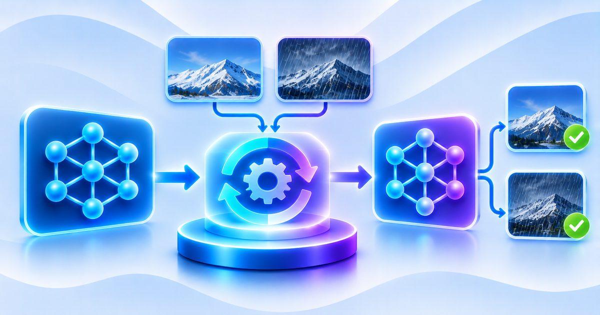
Test-time adaptation is a machine learning approach in which a pretrained model adjusts selected aspects of its behavior using test-time data. The objective is to improve performance on the target distribution without requiring a complete retraining process using the original training pipeline.
The central idea is that incoming data contains information about the environment in which the model is operating. Even when labels are unavailable, the model may be able to use properties such as prediction consistency, feature statistics, reconstruction quality, or self-supervised learning signals to make useful adjustments.
A conventional inference pipeline can be represented as:
[
\hat{y} = f_{\theta}(x)
]
The model receives input (x), applies fixed parameters (\theta), and produces prediction (\hat{y}).
In a test-time adaptation pipeline, the model first or simultaneously updates an adaptation state:
[
\theta_t = \operatorname{Adapt}(\theta_{t-1},x_t)
]
The prediction is then generated using the adapted parameters:
[
\hat{y}t = f{\theta_t}(x_t)
]
The exact sequence depends on the adaptation method. Some methods update parameters using a batch before producing predictions for that batch. Others use a prediction to calculate an adaptation objective and update the model for subsequent inputs. This distinction is important when comparing offline batch adaptation with strict online adaptation.
Unlike conventional supervised retraining, many TTA approaches do not require target labels. They instead optimize an unsupervised or self-supervised objective. For example, a model may reduce the entropy of its predictions, align feature statistics, or encourage consistency across different transformations of the same input.
A widely studied approach is Tent, introduced in the ICLR 2021 paper Fully Test-Time Adaptation by Entropy Minimization. Tent adapts normalization statistics and channel-wise affine parameters by minimizing prediction entropy on incoming test batches while keeping most of the network fixed. The research demonstrated improvements on image corruption and domain-adaptation benchmarks without using the original training data during adaptation.
The key distinction is that the model does not need to restart its entire learning process. It reuses its pretrained knowledge and makes controlled changes based on the target environment.
This makes TTA particularly relevant for deployed systems that need to remain responsive to environmental changes. It also connects to the broader engineering challenge of building "Adaptive ML Systems: How Models Respond When the Environment Changes", where adaptation and monitoring become ongoing responsibilities rather than activities performed only during scheduled retraining.
Test-Time Adaptation Versus Retraining, Fine-Tuning, and Domain Adaptation
Test-time adaptation is related to several established machine learning approaches, but the methods differ in their assumptions, available data, and deployment requirements.
Full retraining generally means rebuilding a model using a training dataset that may include newly collected examples. It can update all model parameters and potentially change the architecture, training objective, or feature-processing pipeline. Although retraining provides substantial flexibility, it requires data preparation, training infrastructure, evaluation, and deployment coordination.
Fine-tuning starts with an existing pretrained model and continues training it on a new dataset. It can be supervised or unsupervised, depending on the available data and learning objective. Fine-tuning often requires a prepared target dataset and a deliberate optimization process, while TTA is typically designed to operate directly on incoming test data.
Domain adaptation generally aims to transfer knowledge from a source domain to a target domain. Some domain-adaptation methods use labeled source data and unlabeled target data, while others operate without source examples. Test-time adaptation is a more deployment-oriented setting in which the model adapts using information available during testing, often without access to source data or target labels.
Online learning is a broader concept involving model updates as new data arrives. It can use labeled feedback, delayed outcomes, or explicit supervision. Online TTA is a specific form of adaptation that typically relies on unlabeled test inputs and self-supervised objectives.
The distinction becomes clearer when considering operational constraints. A company might periodically retrain a fraud model using newly labeled transaction data. It might fine-tune a pretrained vision model using a curated dataset from a new camera environment. Alternatively, it might deploy a TTA mechanism that adjusts selected model parameters as unlabeled images arrive from that camera.
Each approach solves a different problem. Retraining is appropriate when the underlying task or learned relationships require substantial revision. Fine-tuning is useful when a target dataset can be collected and processed. TTA is useful when adaptation must happen during deployment with limited access to labels or source data.
These techniques can also work together. A production system may use test-time adaptation for short-term environmental changes while collecting validated examples for periodic retraining. The adaptation layer provides responsiveness, while the retraining pipeline provides a more comprehensive opportunity to update the model's knowledge.
Key Takeaway
Test-time adaptation addresses a fundamental weakness of static machine learning deployment: the assumption that production data will always resemble training data. By using unlabeled or self-supervised information from incoming inputs, a pretrained model can adjust selected parameters or representations without a complete retraining cycle. However, batch, online, and continual adaptation have different operational requirements, and the right approach depends on how quickly the environment changes, whether labels are available, and how much adaptation overhead the application can tolerate.
Section 2: Real-World Applications of Test-Time Adaptation
Computer Vision, Robotics, and Autonomous Systems
Computer vision systems frequently encounter environmental conditions that differ from those represented in their training datasets. Changes in lighting, weather, camera hardware, image resolution, and sensor positioning can affect image statistics and model performance.
An object detection model trained using clear daytime road images may struggle when deployed during heavy rain or at night. A semantic segmentation system may misclassify road boundaries when visibility decreases. A robotic vision system may encounter different surfaces, backgrounds, or lighting conditions when moved from a laboratory to an industrial environment.
Test-time adaptation can help address certain types of these shifts. A model can use incoming unlabeled images to adjust normalization statistics, improve feature alignment, or encourage prediction consistency across transformations. For a video-based system, adaptation can also exploit temporal information across consecutive frames.
Robotics introduces additional complexity because the environment may change continuously as the robot moves. A mobile robot can transition between indoor and outdoor environments, encounter different illumination conditions, or experience changes in camera viewpoint. An adaptive perception system may need to update its representation without interrupting the robot's real-time operation.
Autonomous driving is another important application. A deployed perception system may encounter weather conditions, camera characteristics, road surfaces, and regional environments that were underrepresented during training. TTA offers a mechanism for adjusting the model using unlabeled observations from the current environment.
However, these applications require particularly strict safety controls. An incorrect adaptation can cause the model to become less reliable in a safety-critical situation. The system must be able to detect unstable updates, retain a known-good model, and fall back to conservative behavior when confidence in adaptation is insufficient.
A useful architecture separates the adaptation process from safety-critical decision logic. The adaptive model can propose updated predictions, while downstream validation and safety mechanisms determine whether those predictions are suitable for action.
TTA should therefore be viewed as one component of a robust perception system rather than a replacement for sensor validation, redundancy, safety monitoring, or comprehensive testing.
Medical Imaging and Healthcare AI
Medical imaging systems are often deployed across hospitals, diagnostic centers, and clinical environments with different scanners, acquisition protocols, imaging parameters, and patient populations. These differences can introduce domain shifts even when the underlying medical task remains unchanged.
For example, an image segmentation model trained using scans from one scanner manufacturer may encounter images from another manufacturer with different intensity distributions or acquisition characteristics. A model developed using a particular imaging protocol may also experience reduced performance when the protocol changes.
Test-time adaptation can help a pretrained model adjust to certain scanner- or environment-specific differences using unlabeled target images. It may update normalization statistics, align feature distributions, or use consistency objectives to improve predictions.
This is particularly relevant when labeled medical data is expensive to obtain. Producing reliable labels may require specialist clinicians, detailed annotation guidelines, and substantial review. In contrast, unlabeled images may already be available within the clinical workflow.
However, the availability of unlabeled data does not mean that adaptation can proceed without oversight. A model can produce confident but incorrect predictions, and changes in patient populations may represent more than simple image-style differences. A change in disease prevalence or the relationship between imaging features and clinical outcomes may require validated labels and a more comprehensive model update.
Clinical systems also need reproducibility. Engineers must be able to determine which model version generated a prediction, which adaptation updates were applied, and whether the adapted model passed the required validation procedures.
A practical strategy is to use test-time adaptation as a controlled technical mechanism within a clinically governed workflow. The system can adapt to carefully defined acquisition shifts, while clinical validation, independent performance evaluation, and appropriate regulatory requirements remain in place.
Fraud Detection, Recommendation Systems, and Industrial Monitoring
Many production prediction systems operate in environments where data characteristics evolve continuously. Fraud detection, recommendation, demand forecasting, and industrial monitoring are examples in which historical patterns may become less representative over time.
A fraud detection model may encounter new transaction behaviors, changes in payment methods, or evolving attack strategies. A recommendation system may observe changes in user preferences, seasonal behavior, and product popularity. An industrial monitoring model may receive sensor readings affected by equipment aging, calibration changes, or environmental conditions.
Test-time adaptation may help a model respond to some of these changes without waiting for a full retraining cycle. For example, a system may update selected representations or normalization statistics when incoming data shows a consistent shift in input characteristics.
However, these applications expose an important limitation of unsupervised adaptation. In many classification problems, the most important changes occur in the relationship between inputs and labels rather than only in the input distribution.
A fraud detection model that sees a new transaction pattern cannot automatically determine whether the pattern represents legitimate behavior or a new fraud strategy without reliable outcome information. Similarly, a recommendation model cannot establish that a change in user behavior reflects a genuine preference unless it receives appropriate feedback.
In such settings, TTA may be useful for handling certain input-level shifts, but it cannot replace outcome-based learning and periodic supervised updates. Delayed labels, customer feedback, confirmed fraud reports, and maintenance records remain important sources of evidence.
An effective production strategy can combine several mechanisms. Test-time adaptation handles short-term distribution changes, monitoring detects changes in model performance, and a retraining pipeline uses validated outcomes to update the model's underlying knowledge.
This is particularly important for streaming systems, where data arrives continuously and the model must make predictions under changing conditions. The engineering concepts are closely related to "Streaming Machine Learning: Building Models That Learn From Data in Real Time", although streaming learning and test-time adaptation remain distinct approaches with different assumptions about supervision and model updates.
Key Takeaway
Test-time adaptation has potential applications in computer vision, robotics, medical imaging, speech recognition, NLP, fraud detection, recommendation systems, and industrial monitoring. Its usefulness depends on the nature of the distribution shift and the reliability of the available adaptation signal. It is most appropriate when incoming data contains useful information about the new environment, while changes in the underlying input-label relationship may still require validated feedback and conventional retraining.
Section 3: Engineering Challenges and Production Deployment
Preventing Catastrophic Forgetting and Adaptation Collapse
One of the most important challenges in test-time adaptation is catastrophic forgetting. As a model adjusts to a new target distribution, it may lose useful knowledge acquired during its original training.
Imagine an image classifier trained to recognize several categories under diverse conditions. During deployment, it receives a long sequence of images from a single environment. An adaptation mechanism updates the model to improve performance on that environment, but the updates gradually weaken its ability to recognize examples from other environments.
This problem becomes more serious in continual adaptation. The model may move through several target distributions over time, with each adaptation step influencing the next. Errors can accumulate, and the model may eventually become highly specialized to recent observations.
Another failure mode is adaptation collapse. A model may begin producing nearly identical predictions for many unrelated inputs. This can happen when unreliable pseudo-labels or unstable optimization updates push the model toward a trivial solution.
The problem is especially relevant to entropy minimization. If a model becomes increasingly confident in an incorrect class, its entropy can decrease even while its actual accuracy deteriorates.
Several strategies can reduce these risks. Parameter restoration moves selected weights toward their original pretrained values. Weight averaging can produce more stable model updates. Teacher-student frameworks provide a reference prediction that is less sensitive to individual noisy examples. Sample filtering prevents unreliable inputs from influencing the adaptation objective.
CoTTA uses stochastic restoration to preserve part of the original model knowledge during continual adaptation. EATA uses regularization to protect important parameters and avoid unnecessary updates. SAR focuses on reliable samples and flatter optimization solutions to improve stability. These methods illustrate different ways to control adaptation rather than allowing unrestricted parameter changes.
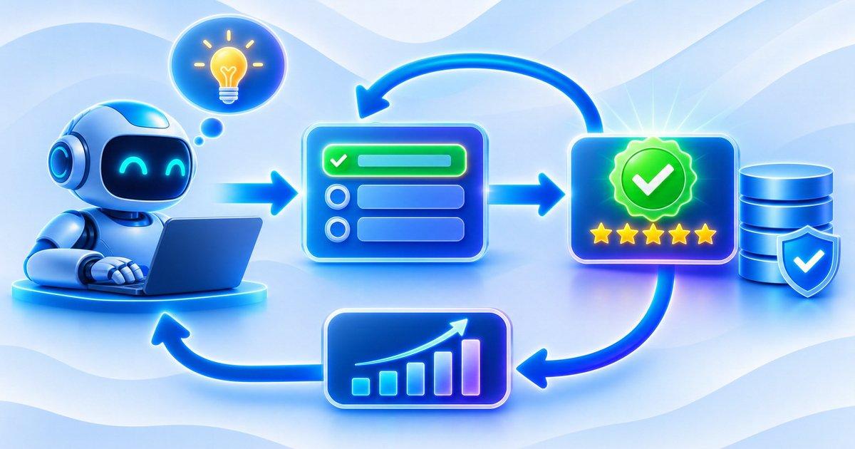
Production systems should also maintain a known-good model checkpoint. If adaptation metrics indicate instability, the system should be able to revert to a previously validated model rather than continuing to apply updates.
Computational Overhead, Latency, and Memory Constraints
Conventional inference usually requires a forward pass through the model. Test-time adaptation may require additional operations, including gradient computation, backward propagation, multiple augmented views, optimization steps, and model-state management.
These operations increase computational cost. In real-time applications, the added latency can be a serious limitation. An autonomous perception system cannot spend an arbitrary amount of time adapting to every incoming frame. A speech recognition service may need to process audio under strict latency requirements. An edge device may not have enough memory to store additional model copies or intermediate activations.
The cost depends on the adaptation method. Updating only normalization statistics may be relatively inexpensive, while adapting many network parameters requires more computation and memory. Teacher-student methods may provide additional stability but introduce overhead from maintaining reference predictions or model states.
The online adaptation survey published in the International Journal of Computer Vision in 2025 emphasizes the importance of evaluating not only accuracy but also computational efficiency, including GPU operations, wall-clock time, and memory consumption. It also highlights the sensitivity of several methods to batch size.
Engineers should therefore measure adaptation overhead as part of model evaluation. Important metrics include additional inference latency, adaptation time per sample or batch, memory consumption, GPU utilization, throughput, and energy consumption on the target hardware.
A practical implementation can use several optimization strategies. The system can update only selected layers, skip redundant samples, limit the number of optimization steps, use smaller adaptation modules, or perform adaptation asynchronously when the application permits it.
Another option is to separate prediction and adaptation workloads. A stable model can continue serving predictions while an adaptation process evaluates candidate updates in parallel. The updated model can be promoted only after passing predefined validation checks.
This architecture is more complex than a single-model inference service, but it creates a clearer boundary between prediction availability and experimental adaptation.
Monitoring, Evaluation, and Safe Deployment
Evaluating a test-time adaptation system requires more than measuring accuracy on a single shifted dataset. Engineers must determine whether the model improves under distribution shift, preserves performance on familiar data, and remains stable over time.
A reliable evaluation strategy should begin with a baseline model that does not adapt. The same pretrained model should then be evaluated under identical target conditions with the adaptation mechanism enabled. This makes it possible to measure the actual contribution of adaptation rather than confusing it with differences in data or evaluation procedures.
Performance should be measured across multiple shift types. These may include changes in image corruption, lighting, sensor characteristics, class proportions, and real-world domain differences. Where possible, evaluation should include both stationary and changing target distributions.
Accuracy alone is insufficient. Depending on the application, useful metrics may include precision, recall, F1 score, calibration error, false-positive rate, and task-specific performance measures. For online systems, latency and memory consumption should also be measured.
A particularly important requirement is to evaluate both shifted and unshifted data. A model may improve performance on the target environment while damaging its original capabilities. This trade-off is central to understanding catastrophic forgetting.
Production monitoring should track adaptation behavior as well as prediction behavior. Relevant signals include changes in prediction entropy, class distribution, feature statistics, update magnitude, gradient norms, and disagreement between the adaptive model and a stable reference model.
These measurements do not independently prove that the model is correct. They are indicators that can help identify unusual behavior and trigger additional checks.
A safe deployment strategy should begin with shadow or recommendation mode. The adaptation mechanism can generate candidate updates without immediately replacing the production model. Engineers can compare its predictions against the existing model and evaluate its behavior on a controlled dataset.
Once the system demonstrates stable performance, limited adaptation can be enabled for selected workloads. Promotion criteria should be explicit, and rollback should remain available.
The validation process should also account for data privacy and security. Test-time adaptation may process sensitive customer, medical, or operational data. The system must follow appropriate data-access policies and ensure that updates cannot be manipulated through malicious or corrupted inputs.
These practices align with broader production ML testing principles described in "ML Testing for Software Engineers: How to Test Systems That Don't Always Produce the Same Output". Adaptive systems require additional testing because their behavior changes as model state changes over time.
Key Takeaway
Production test-time adaptation must address catastrophic forgetting, unstable pseudo-labels, latency, memory consumption, monitoring, and rollback. Reliable systems preserve a known-good model, constrain the parameters that can change, evaluate candidate updates, and maintain a complete adaptation history. The objective is not simply to make a model adapt faster, but to make every adaptation decision measurable, controlled, and reversible.
Conclusion
Test-time adaptation represents an important shift in how machine learning systems can operate after deployment. Traditional inference assumes that a trained model remains fixed, even when the data distribution changes. TTA challenges that assumption by allowing a model to use incoming test data to adjust selected parameters, normalization statistics, or representations without requiring a complete retraining process.
Techniques such as entropy minimization, normalization updates, pseudo-labeling, consistency learning, and parameter-efficient adaptation provide different ways to extract useful learning signals from unlabeled data. Methods including Tent, EATA, CoTTA, SAR, and EcoTTA demonstrate how researchers are addressing the central challenges of adaptation effectiveness, efficiency, and stability.
The applications extend across computer vision, robotics, medical imaging, speech recognition, NLP, fraud detection, recommendation systems, and industrial monitoring. In these environments, models may encounter new input conditions long before a conventional retraining cycle can produce an updated version.
However, test-time adaptation is not a universal replacement for retraining. It cannot reliably correct every form of distribution shift, particularly when the relationship between inputs and labels changes substantially. Unlabeled data can provide useful information about the target environment, but it cannot always reveal whether a prediction is correct.
For engineering teams, the challenge is to build adaptation mechanisms that improve responsiveness without sacrificing reliability. This requires careful selection of adaptation objectives, parameter restrictions, uncertainty monitoring, computational budgets, validation procedures, and rollback mechanisms.
The future of production machine learning is likely to combine several approaches. Monitoring systems will identify changing conditions, test-time adaptation will provide controlled short-term adjustments, and periodic retraining will incorporate validated new information into the model's underlying knowledge.
The most effective machine learning systems will not necessarily be those that update themselves continuously. They will be systems that know when adaptation is useful, which information is trustworthy, how much change is safe, and when a more comprehensive model update is necessary.
Frequently Asked Questions
1. What is test-time adaptation in machine learning?
Test-time adaptation is a technique that allows a pretrained machine learning model to adjust selected parameters or internal statistics using incoming test data. It is designed to improve performance when production data differs from the training distribution, often without requiring target labels or access to the original training dataset.
2. How does test-time adaptation work without retraining?
TTA uses unsupervised or self-supervised objectives derived from incoming data to update selected parts of an existing model. Instead of rebuilding the complete model, it may adjust normalization statistics, optimize selected parameters, or improve prediction consistency.
3. What is the difference between test-time adaptation and fine-tuning?
Fine-tuning typically continues training a pretrained model using a prepared target dataset, which may contain labeled or unlabeled examples. Test-time adaptation is generally designed to operate directly on test inputs during deployment, often without ground-truth labels or access to the original training data.
4. What is entropy minimization in test-time adaptation?
Entropy minimization reduces the uncertainty of a model's predictions on incoming test data. It is used as an unsupervised optimization objective in methods such as Tent, but lower prediction entropy does not necessarily mean higher accuracy because a model can become confidently incorrect.
5. What is the Tent method?
Tent stands for Fully Test-Time Adaptation by Entropy Minimization. It adapts normalization statistics and affine parameters using incoming target data while keeping most of the pretrained model fixed, allowing the model to respond to distribution shifts without conventional retraining.
6. What is continual test-time adaptation?
Continual test-time adaptation allows a model to adjust as data distributions change repeatedly over time. It is designed for long-running deployments where the model may encounter multiple environments rather than one fixed target distribution.
7. Does test-time adaptation require labeled data?
Many TTA methods operate without labeled target data. They use objectives such as entropy minimization, pseudo-labeling, self-supervised learning, and prediction consistency, although reliable labeled evaluation data remains important for measuring actual model accuracy.
8. What is catastrophic forgetting in test-time adaptation?
Catastrophic forgetting occurs when adapting to new data damages knowledge learned during the original training process. A model may improve on one target environment while losing performance on previously supported environments, making parameter restoration and regularization important safeguards.
9. What is the difference between online and batch test-time adaptation?
Batch TTA adapts using a collection of target examples available together, while online TTA processes incoming examples or batches sequentially. Online adaptation is often more suitable for real-time systems but introduces additional challenges involving small batches, latency, and update stability.
10. Can test-time adaptation improve computer vision models?
Yes. TTA can help computer vision models respond to changes in lighting, weather, camera characteristics, and image quality. Its effectiveness depends on whether the distribution shift can be addressed using the available unlabeled data and adaptation objective.
11. Is test-time adaptation suitable for large language models?
Some adaptation ideas can be applied to language models, including parameter-efficient updates, prompt adaptation, and inference-time learning. However, changing prompts or retrieval context is not necessarily the same as gradient-based test-time adaptation, so the exact adaptation mechanism must be distinguished.
12. What are the main challenges of test-time adaptation?
The main challenges include noisy pseudo-labels, catastrophic forgetting, adaptation collapse, computational overhead, small-batch instability, and difficulty evaluating accuracy without target labels. Production systems must also address privacy, security, monitoring, and rollback.
13. How can engineers prevent a model from becoming unstable during test-time adaptation?
Engineers can use sample filtering, learning-rate controls, parameter restrictions, regularization, teacher-student models, and parameter restoration. Maintaining a known-good model checkpoint and monitoring adaptation behavior are also important for detecting and reversing harmful updates.
14. Does test-time adaptation replace model retraining?
No. TTA is useful for controlled adjustments to certain distribution shifts, but it cannot reliably learn every new relationship or correct every form of concept drift without validated feedback. Periodic retraining remains necessary when the underlying task, labels, or learned relationships change substantially.
15. What is the future of test-time adaptation?
Future research is likely to focus on more efficient continual adaptation, parameter-efficient learning, stronger uncertainty estimation, adaptation for foundation models, and better evaluation under realistic distribution shifts. Production systems will increasingly combine test-time adaptation with monitoring, feedback collection, and scheduled retraining.