Forecasting Infrastructure Demand With Machine Learning: From Metrics to Capacity Planning

Section 1: Turning Infrastructure Metrics Into a Workload Forecasting Problem

Understanding What Infrastructure Metrics Reveal About Actual Demand

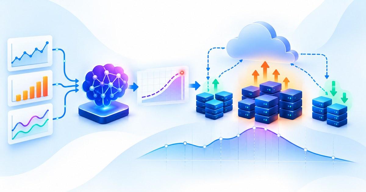
Modern applications generate continuous streams of infrastructure telemetry that reveal how workloads consume computing resources, how traffic changes over time, and where operational bottlenecks emerge. Metrics such as CPU utilization, memory consumption, request throughput, network bandwidth, disk activity, and queue depth help engineers understand current system behavior, but their greatest value for capacity planning comes from identifying relationships between application demand and the resources required to serve it reliably. By analyzing these measurements alongside application-level indicators, engineering teams can develop a more complete picture of infrastructure requirements instead of relying on isolated utilization thresholds or historical averages.

For example, a backend API may experience increasing request volume while maintaining relatively stable CPU utilization because its existing instances still have sufficient processing capacity, whereas a background data-processing service may develop growing message queues even when its average CPU consumption appears moderate. These situations demonstrate why individual infrastructure metrics cannot always explain workload pressure independently, particularly when applications depend on databases, external APIs, shared storage, or asynchronous processing pipelines. Engineers should therefore connect infrastructure telemetry with request rates, concurrent users, queue growth, response latency, and dependency performance to understand how changes in application activity translate into resource requirements.

Historical telemetry also provides evidence about how workloads behave under different operating conditions, including routine traffic fluctuations, scheduled jobs, deployment events, and recurring periods of high demand. When these observations are recorded consistently over time, machine learning models can learn patterns that help estimate future workload levels, while engineering teams can use the resulting forecasts to make more informed capacity decisions. However, forecasts are only as useful as the measurements and assumptions supporting them, making reliable instrumentation, consistent sampling intervals, and clear definitions of monitored metrics essential foundations for infrastructure demand forecasting.

Connecting Request Rates, Resource Utilization, and Application Workloads

Forecasting infrastructure demand requires understanding the relationship between incoming workload and the resources needed to process it, because request volume alone does not determine how much computing capacity an application will consume. A thousand lightweight API requests may require substantially less compute than the same number of requests involving complex database queries, large payloads, or computationally expensive model inference. Engineers therefore need to analyze historical relationships between workload indicators and resource consumption, allowing forecasting systems to estimate not only how much activity is expected but also how that activity may translate into CPU, memory, storage, network, and concurrency requirements.

This relationship can be difficult to model when applications contain multiple services with different processing characteristics or when a workload changes its resource profile over time. For instance, a deployment that introduces additional data transformation steps may increase CPU consumption per request even if incoming traffic remains unchanged, while a new caching layer may reduce database utilization without changing the number of user requests. Capacity forecasting should therefore account for relevant application changes, service-level resource profiles, and the dependencies that influence workload execution, rather than assuming that historical traffic and infrastructure utilization always maintain a fixed relationship.

Combining infrastructure metrics with application-level signals can improve the usefulness of capacity forecasts by helping models distinguish between increased demand and changes in how efficiently a system processes that demand. Request throughput, latency percentiles, queue depth, and concurrency can reveal workload pressure that average utilization metrics may not capture, while deployment records and application logs provide additional context for interpreting changes in resource consumption. This approach aligns with Machine Learning for Log Analytics: Turning Application Logs Into Predictive Signals, which explores how operational data can help engineering teams identify patterns and extract actionable insights from production systems. 

Identifying Seasonality, Traffic Bursts, and Long-Term Growth Patterns

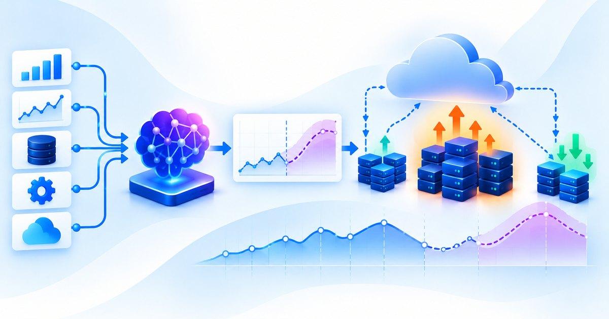
Infrastructure workloads often exhibit recurring temporal patterns that provide useful signals for forecasting future resource requirements, including daily traffic cycles, weekly business activity, scheduled batch processing, and seasonal demand changes. A business application may experience higher request volumes during working hours, while an online retail platform may encounter predictable increases during promotional periods or major shopping events. By examining historical telemetry across appropriate time windows, forecasting models can learn these repeating patterns and estimate when infrastructure demand is likely to rise or fall, helping engineering teams distinguish recurring workload behavior from short-lived fluctuations.

Traffic bursts introduce a different forecasting challenge because sudden increases may develop more quickly than infrastructure can be provisioned and initialized. A viral product launch, an unexpected external integration event, or a rapid increase in automated traffic can produce demand that differs substantially from historical patterns, making it difficult for a model trained primarily on regular workloads to anticipate the full scale of the change. Engineers should therefore examine peak-demand behavior separately from average workload conditions, combining historical forecasts with real-time monitoring and operational safeguards so that the capacity planning process does not depend entirely on the assumption that future demand will resemble the past.

Long-term growth also matters because an application with gradually increasing traffic may require additional capacity even when its daily or weekly usage pattern remains stable. Tracking sustained changes in request volume, data ingestion rates, active users, and resource consumption can help teams distinguish structural growth from temporary peaks, while comparing these trends with application releases and business activity can provide useful context for capacity planning. A robust forecasting approach should therefore consider recurring seasonality, short-term spikes, and longer-term growth together, allowing engineering teams to plan for both immediate workload changes and the gradual expansion of infrastructure requirements over time.

Key Takeaway

Forecasting infrastructure demand begins with reliable telemetry and a clear understanding of how application workloads translate into resource consumption. By combining infrastructure metrics with request-level signals, identifying recurring patterns and long-term growth, and defining explicit prediction horizons and capacity objectives, engineering teams can turn historical observations into actionable forecasts. The goal is not simply to predict future metrics, but to estimate the resources required to maintain application performance and reliability while making informed decisions about infrastructure capacity and cost.

Section 2: Building Machine Learning Models That Forecast Infrastructure Demand

Preparing Historical Metrics for Time-Series Forecasting

Building a reliable infrastructure demand forecasting model begins with preparing historical telemetry so that the data accurately represents how workloads evolve over time. Metrics such as CPU utilization, memory consumption, request throughput, network activity, and queue depth are typically collected through monitoring systems, but raw observations may contain missing values, duplicate records, irregular sampling intervals, or temporary spikes caused by instrumentation problems. Before training a forecasting model, engineers must identify these issues, standardize timestamps, align metrics collected at different frequencies, and distinguish genuine workload changes from measurement errors that could distort future predictions.

Time-series preparation also requires preserving the chronological order of observations because infrastructure forecasting depends on understanding how previous conditions relate to subsequent workloads. Randomly shuffling historical metrics before splitting training and evaluation datasets can allow information from future periods to influence model development, producing unrealistically optimistic results that do not reflect the uncertainty encountered during production forecasting. A more reliable approach uses chronological training, validation, and testing windows, allowing engineers to assess how well a model trained on earlier observations predicts workloads occurring later, particularly when traffic patterns and resource consumption change over time.

Feature engineering can further improve forecasts by representing temporal relationships that are not immediately visible in individual metric values, including rolling averages, recent growth rates, lagged observations, hour-of-day effects, day-of-week patterns, and the relationship between request volume and resource utilization. For example, a model forecasting weekday CPU demand may benefit from knowing the current utilization, recent traffic growth, and historical usage during comparable periods, while a data-processing workload may require features describing queue accumulation and scheduled job execution. Engineers should also account for deployment changes and changes in service configuration because an application update can alter resource consumption even when incoming traffic remains relatively stable, making historical observations less representative of the current system.

Choosing Between Statistical Forecasting and Machine Learning Models

Statistical forecasting methods provide a useful starting point for infrastructure demand prediction because many workloads exhibit temporal patterns that can be captured without introducing complex model architectures. Exponential smoothing can represent certain trends and seasonal patterns, while autoregressive models and related time-series techniques can capture relationships between current observations and earlier values. These methods are often practical baselines when workloads are relatively stable and engineers need forecasts that are straightforward to evaluate and operate, although their suitability depends on the characteristics of the metrics and the prediction horizon.

Machine learning models become useful when infrastructure demand depends on multiple interacting signals that are difficult to represent through a single time series or a simple statistical relationship. Tree-based approaches, including gradient-boosted decision trees, can combine request volume, time-related features, recent utilization, workload categories, and deployment indicators to estimate future resource consumption, while neural forecasting models may capture more complex temporal patterns when sufficient representative data is available. However, greater model complexity does not automatically produce better forecasts, particularly when historical telemetry is limited, workload behavior changes frequently, or the computational cost of maintaining the forecasting pipeline exceeds the benefit of more sophisticated predictions.

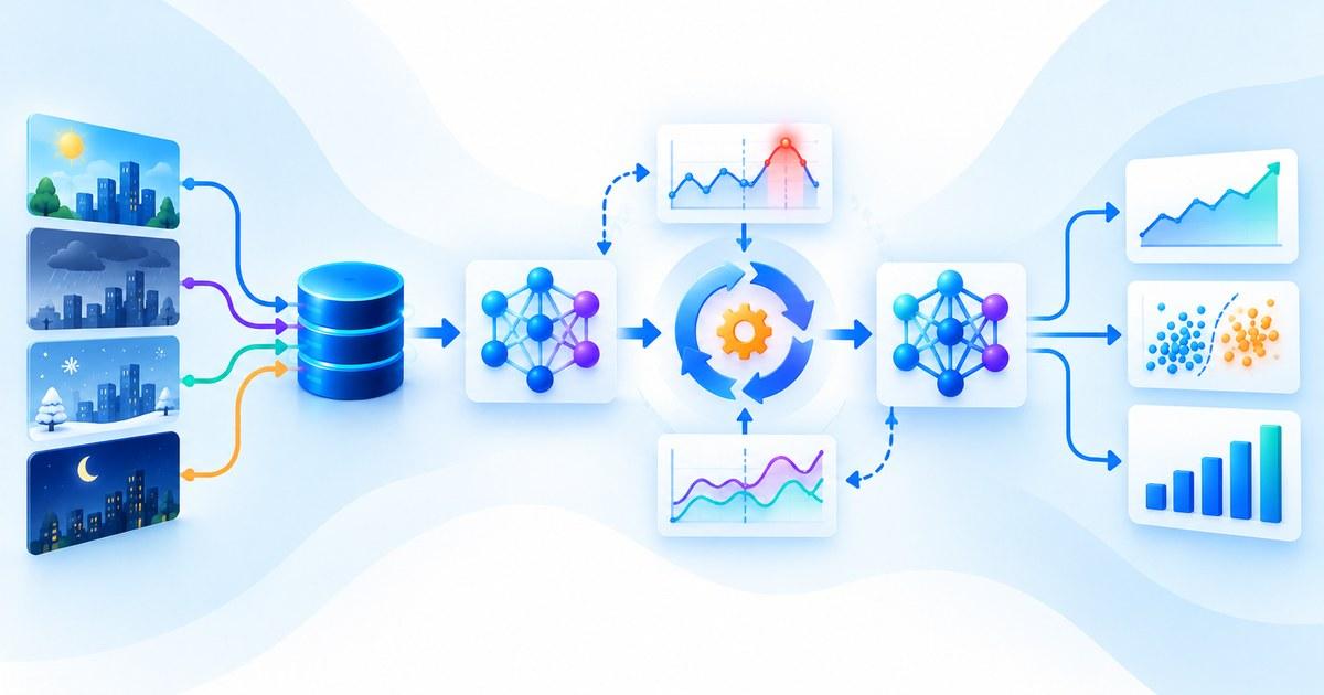
Model selection should therefore begin with a simple baseline and progress toward more complex approaches only when evaluation demonstrates a meaningful improvement for the intended capacity planning task. A model forecasting CPU utilization for the next few minutes may require different assumptions from a model estimating memory demand over the next several days, because the two predictions support different operational decisions and face different sources of uncertainty. The principles explored in “Adaptive ML Systems: How Models Respond When the Environment Changes” are relevant when selecting and maintaining these models, since changes in workload behavior can undermine previously reliable forecasts and require teams to reassess model suitability over time.

Combining Multiple Signals to Predict Future Resource Requirements

Infrastructure demand is influenced by several connected variables, making multivariate forecasting valuable when individual metrics cannot adequately represent the workload's behavior. Incoming request volume, active connections, queue depth, CPU utilization, memory pressure, cache activity, and downstream service latency may each provide different evidence about how an application is likely to consume resources in the future. By combining these signals, engineers can develop forecasts that account for changes in workload intensity as well as variations in how efficiently the application processes that workload.

For example, a backend service may experience an increase in incoming requests while CPU utilization remains moderate because existing instances still have sufficient capacity, whereas a rapidly growing queue may indicate that processing demand is beginning to exceed the rate at which work can be completed. A forecasting model that considers request rates alongside queue growth and resource consumption may provide a more informative estimate of upcoming pressure than one trained on CPU utilization alone. Similarly, a workload that frequently retrieves large datasets or performs computationally expensive transformations may require features describing request complexity or processing volume, helping the system distinguish between traffic increases that have similar request counts but very different resource implications.

Combining signals also requires attention to temporal alignment, feature availability, and dependencies between services, because metrics collected at different intervals may not describe the same operational period. Engineers should determine whether each input is available at the time a forecast is generated, validate the relationship between its historical values and the prediction target, and avoid incorporating information that would only become observable after the forecast period. In addition, correlations between metrics should be interpreted carefully because an increase in memory consumption or latency may be a consequence of existing resource pressure rather than an independent indicator of future demand, making domain knowledge and evaluation essential when selecting features for a forecasting model.

Key Takeaway

Building useful infrastructure demand forecasting models requires reliable historical telemetry, chronological data preparation, appropriate model selection, and evaluation across both ordinary workloads and peak-demand conditions. Combining multiple operational signals can improve forecasts when those signals explain how application activity translates into resource consumption, while careful temporal validation helps prevent misleading results caused by future information or unrepresentative test data. By assessing forecasts according to their impact on actual capacity decisions, engineering teams can identify models that help maintain application performance while managing infrastructure utilization and cost.

Section 3: Translating Workload Forecasts Into Infrastructure Capacity Plans

Converting Predicted Workload Into CPU, Memory, and Compute Requirements

Forecasting infrastructure demand becomes operationally useful when predicted workload levels are translated into concrete resource requirements that engineering teams can use for capacity planning. A model might estimate that an application will receive 40% more requests during the next hour, but that forecast alone does not establish how many additional instances, CPU cores, or memory resources will be required, because the answer depends on the processing cost of each request, current system utilization, and the performance targets the application must maintain. Engineers should therefore combine workload forecasts with historical throughput measurements, resource consumption profiles, and application performance benchmarks to estimate the capacity needed under the predicted conditions.

For example, a backend service that handles lightweight API requests may accommodate increased traffic by adding a small number of application replicas, whereas a service that performs computationally expensive data transformations may require substantially more CPU capacity for the same increase in request volume. Memory planning introduces additional considerations because resource consumption may depend on cached data, concurrent requests, intermediate processing objects, and the size of models loaded into memory, while workloads involving machine learning inference may also depend on GPU availability and accelerator memory. By measuring how resource consumption changes across different workload levels, engineers can build capacity models that connect predicted demand with the computational resources required to meet service-level objectives.

These relationships should be reassessed when application code, model architectures, feature processing, or infrastructure configurations change, since historical resource profiles may no longer represent the current system. Combining forecasting outputs with recent performance measurements and controlled load tests allows capacity planners to estimate resource requirements more realistically than simply extending historical utilization trends, while the principles discussed in “Resource-Aware Machine Learning: Designing Models Around Compute and Energy Limits” provide useful context for matching computational resources to workload characteristics.

Estimating Capacity Headroom, Provisioning Time, and Service Limits

Infrastructure capacity plans must account for the difference between the resources a workload is expected to consume and the capacity that should actually be available to maintain reliable operation under changing conditions. Provisioning exactly enough resources to match a forecast can leave an application exposed to performance degradation when predictions underestimate demand, processing costs increase unexpectedly, or workload bursts occur before additional capacity becomes available. Engineers therefore establish capacity headroom through explicit utilization targets and safety margins, balancing the need to absorb demand fluctuations against the financial cost of maintaining unused resources.

Provisioning time is equally important because a capacity forecast is useful only when it arrives early enough for the required infrastructure to become operational. A containerized application may require time to schedule new replicas, download images, initialize dependencies, populate caches, and pass readiness checks, while a workload requiring specialized accelerators or additional cloud resources may face longer provisioning delays or resource availability constraints. Capacity planning should therefore align the forecast horizon with measured startup and readiness times, allowing teams to determine when additional resources must be requested to support the expected workload rather than waiting until utilization approaches its limit.

Resource quotas and service limits also constrain what a capacity plan can achieve, particularly when several workloads compete for shared compute, memory, network, or cloud capacity. An accurate forecast cannot guarantee that additional resources will be immediately available when cloud quotas, cluster limits, or downstream service constraints prevent the application from expanding as expected. By incorporating these restrictions into planning, engineering teams can identify potential capacity shortages earlier, evaluate alternative resource allocations, and establish escalation or fallback procedures for situations in which forecasted demand exceeds the resources that can realistically be provisioned.

Planning Resources Across Services, Clusters, and Cloud Environments

Capacity planning becomes more complicated in distributed applications because workload growth in one service can increase resource demand elsewhere in the system, creating dependencies that cannot be addressed by forecasting each component independently. An increase in API traffic may raise CPU consumption in application replicas, increase database queries, generate more messages for background workers, and create additional demand on shared feature stores or caching infrastructure. If engineers provision extra application capacity without accounting for these dependencies, they may shift the bottleneck to a database or message-processing service, limiting the benefit of the original forecast and potentially worsening end-to-end performance.

A more complete planning approach combines service-level workload forecasts with an understanding of resource dependencies, throughput limits, and current capacity across the broader infrastructure environment. For example, predicted growth in a data-processing workload should be assessed against the capacity of its worker pool, message broker, object storage, and downstream database, allowing engineers to identify which components are likely to constrain throughput during peak periods. In Kubernetes environments, this also involves accounting for pod resource requests and limits, node capacity, scheduling constraints, and cluster autoscaling behavior, while cloud deployments may require additional consideration of regional capacity, instance availability, network limits, and service quotas.

Planning across multiple environments introduces further trade-offs when workloads can run in different clusters, availability zones, or cloud regions, because available resources may differ in cost, performance, and operational suitability. Capacity forecasts can help teams estimate where additional resources will be needed and assess whether workloads should be redistributed, scaled independently, or scheduled during periods of lower demand, provided that such decisions respect data locality, latency requirements, and resilience objectives. By combining workload forecasts with dependency maps and infrastructure inventories, engineers can move from isolated resource estimates toward capacity plans that reflect how the complete application behaves under expected demand.

Key Takeaway

Translating workload forecasts into capacity plans requires connecting predicted demand with measured resource consumption, provisioning delays, shared service dependencies, infrastructure limits, and application reliability objectives. Engineers must account for CPU, memory, and specialized compute requirements while maintaining appropriate headroom for forecast errors and unexpected traffic, ensuring that additional capacity can become available before performance deteriorates. By evaluating resource plans against actual workload behavior, engineering teams can make better-informed decisions that balance service reliability, infrastructure utilization, and cloud expenditure.

Conclusion: From Infrastructure Metrics to Data-Driven Capacity Planning

Forecasting infrastructure demand with machine learning enables engineering teams to move beyond historical averages and reactive resource decisions toward a more informed understanding of how application workloads are likely to evolve. Production telemetry provides valuable evidence about request volume, CPU utilization, memory consumption, queue depth, network activity, and application performance, but these measurements become substantially more useful when analyzed together to uncover recurring patterns and relationships between workload intensity and resource requirements. By transforming operational metrics into reliable forecasts, organizations can make better-informed decisions about infrastructure capacity, cloud expenditure, application performance, and long-term resource planning.

Building a useful forecasting system requires more than selecting a machine learning algorithm, because the quality of its predictions depends on telemetry reliability, temporal data preparation, representative training examples, and evaluation against realistic workload conditions. Statistical forecasting methods may provide sufficient accuracy for relatively stable workloads, while machine learning models can incorporate multiple signals when resource consumption depends on more complex interactions between traffic, application behavior, and infrastructure conditions. Regardless of the chosen approach, engineering teams should evaluate forecasts chronologically and examine their performance across normal workloads, peak-demand periods, and changing operating conditions rather than relying exclusively on aggregate accuracy metrics.

The operational value of forecasting emerges when predictions are translated into practical capacity plans that account for resource consumption, provisioning delays, workload dependencies, service limits, and reliability requirements. An accurate estimate of future request volume does not automatically determine the number of application replicas or the amount of CPU and memory required, since the appropriate capacity also depends on request complexity, throughput per instance, existing utilization, and the consequences of insufficient resources. By connecting workload forecasts with measured resource profiles and application service-level objectives, engineers can estimate capacity requirements more realistically and balance the risks of overprovisioning against the cost of resource shortages.

Production forecasting also requires continuous monitoring because workload patterns, application configurations, and resource-consumption relationships can change after deployment. Engineering teams should compare predicted and observed metrics, investigate systematic forecast errors, detect changes in workload behavior, and periodically reassess whether their forecasting models remain appropriate for current operating conditions. Integrating these forecasts with established infrastructure management processes can support near-term resource adjustments, long-term growth planning, and cloud budget forecasting, while reactive safeguards remain essential for handling unexpected demand and situations that machine learning models cannot anticipate reliably.

Ultimately, the objective of machine learning-based infrastructure forecasting is not simply to predict future metrics with minimal error, but to improve the quality of the resource decisions made from those predictions. Organizations should begin with a measurable capacity planning problem, establish a baseline using their existing forecasting or planning methods, and evaluate whether machine learning delivers meaningful improvements in availability, latency, resource utilization, and total operating cost. By combining reliable telemetry, appropriate forecasting models, realistic capacity calculations, and continuous operational evaluation, engineering teams can build a sustainable approach to infrastructure planning that responds to changing workloads without introducing unnecessary computational expense or operational complexity.

Frequently Asked Questions

1. What Is Infrastructure Demand Forecasting With Machine Learning?

Infrastructure demand forecasting with machine learning uses historical operational metrics and workload information to estimate future infrastructure requirements, including CPU usage, memory consumption, request volume, storage demand, and processing capacity. By identifying recurring patterns and relationships between workload indicators, forecasting models help engineering teams anticipate resource needs and make better-informed capacity planning decisions before demand changes create performance or availability problems.

2. Why Is Infrastructure Demand Forecasting Important?

Infrastructure demand forecasting helps organizations prepare for workload growth, recurring traffic peaks, and changing application requirements before available capacity becomes insufficient. Accurate forecasts can support more effective resource allocation, reduce unnecessary overprovisioning, improve infrastructure budgeting, and help engineering teams maintain application performance, particularly when provisioning additional capacity requires significant time or coordination.

3. Which Infrastructure Metrics Are Most Useful for Demand Forecasting?

Useful metrics include CPU utilization, memory consumption, request throughput, concurrent connections, network activity, disk I/O, queue depth, response latency, and the number of active application instances. The most appropriate combination depends on the workload, since interactive APIs, database systems, background processing pipelines, and ML inference services have different resource-consumption patterns that cannot always be understood through a single utilization metric.

4. What Is the Difference Between Workload Forecasting and Resource Forecasting?

Workload forecasting estimates future application activity, such as incoming requests, transactions, active users, or message volume, whereas resource forecasting estimates the computing resources required to process that activity. Workload predictions can inform resource estimates, but capacity planning must also account for request complexity, resource consumption per unit of work, current capacity, provisioning delays, and the performance objectives the application must satisfy.

5. Which Machine Learning Models Can Forecast Infrastructure Demand?

Infrastructure forecasting can use statistical methods such as exponential smoothing and autoregressive models, as well as machine learning approaches such as gradient-boosted decision trees and neural networks designed for sequential data. The appropriate method depends on the workload's temporal patterns, available telemetry, forecast horizon, computational cost, and required accuracy, making comparison against a simple baseline important before adopting a more complex model.

6. How Much Historical Data Is Needed to Forecast Infrastructure Demand?

The amount of historical data required depends on the workload's variability, seasonal patterns, forecasting horizon, and the complexity of the selected model. A workload with stable daily behavior may be easier to forecast than one influenced by irregular business events or rapid product growth, so engineers should collect enough representative observations to capture relevant operating cycles and evaluate the model against later periods that were not used during training.

7. How Far Into the Future Can Infrastructure Demand Be Forecast?

The useful forecasting horizon depends on how quickly workloads change and how much advance notice engineering teams need to make capacity decisions. Short-term forecasts can support operational resource planning, while longer-term estimates can inform infrastructure expansion and budgeting, although uncertainty generally increases with the horizon and should be reflected in the way forecasts are evaluated and used.

8. How Can Engineers Evaluate Infrastructure Forecast Accuracy?

Engineers can evaluate forecasts using measures such as Mean Absolute Error and Root Mean Squared Error, comparing predicted resource consumption with subsequently observed values across chronological evaluation periods. They should also assess systematic underestimation, peak-demand errors, forecast stability, and performance across different workload conditions, because a model with low average error may still be unsuitable if it consistently misses the demand spikes that threaten application reliability.

9. How Does Machine Learning Help With CPU and Memory Capacity Planning?

Machine learning can identify relationships between workload indicators and historical CPU or memory consumption, allowing engineers to estimate future resource requirements under anticipated operating conditions. These forecasts can be combined with measured instance throughput, application resource profiles, utilization targets, and appropriate safety margins to estimate the capacity needed to maintain performance without relying solely on fixed utilization thresholds or historical averages.

10. How Should Capacity Planning Account for Unexpected Traffic Spikes?

Capacity planning should combine forecasts with adequate resource headroom, measured provisioning times, infrastructure limits, and reactive monitoring that can respond when actual demand exceeds predictions. Because machine learning models cannot anticipate every sudden workload change, engineering teams should also establish fallback procedures, scaling limits, and contingency plans that preserve application reliability when forecasted capacity proves insufficient or additional resources cannot be provisioned immediately.

11. What Is the Difference Between Capacity Forecasting and Predictive Autoscaling?

Capacity forecasting estimates future workload and resource requirements to support planning decisions, while predictive autoscaling uses forecasts to trigger or inform automated infrastructure scaling actions before anticipated demand arrives. Capacity forecasting can support longer-term resource planning, infrastructure budgeting, and workload allocation even when infrastructure changes are performed manually, whereas predictive autoscaling connects demand estimates directly to operational mechanisms that provision or remove resources.

12. How Can Infrastructure Forecasting Help Reduce Cloud Costs?

Infrastructure forecasting can help reduce cloud costs by identifying future resource requirements more accurately, allowing organizations to limit unnecessary spare capacity while maintaining sufficient resources for expected demand. However, cost savings are not guaranteed, since inaccurate predictions, overly conservative safety margins, or the cost of maintaining the forecasting pipeline can offset the benefits, making it important to compare total expenditure and reliability outcomes against existing capacity planning methods.

13. How Should Engineering Teams Handle Changes in Workload Patterns?

Engineering teams should continuously compare predicted and observed demand, investigate systematic forecast errors, and monitor whether application deployments or external conditions have changed the relationship between workload indicators and resource consumption. When the existing forecasting model becomes less reliable, teams may need to revise features, retrain the model, select a different forecasting method, or correct telemetry problems before using new predictions to inform important capacity decisions.

14. Can Infrastructure Demand Forecasting Be Used With Kubernetes and Cloud Platforms?

Yes, infrastructure forecasts can support Kubernetes and cloud capacity planning by estimating workload growth, CPU and memory requirements, and expected resource pressure across services or clusters. Forecasts can inform planning and autoscaling integrations, but the implementation must account for pod resource requests and limits, node capacity, scheduling constraints, cloud quotas, provisioning delays, and the behavior of existing reactive scaling mechanisms rather than assuming predicted workload directly determines the required infrastructure configuration.

15. What Are the Best Practices for Implementing Infrastructure Demand Forecasting in Production?

A reliable implementation begins with consistent telemetry collection, clearly defined forecasting targets, chronological model evaluation, and a measurable capacity planning objective that reflects application performance and cost requirements. Engineering teams should establish a baseline using existing methods, monitor prediction errors and workload drift, translate forecasts into resource requirements using measured capacity profiles, and retain reactive safeguards for unexpected demand, ensuring that machine learning improves real infrastructure decisions rather than optimizing forecasting accuracy without measurable operational benefits.