
Section 1: Why Traditional Autoscaling Struggles With Unpredictable Infrastructure Demand
Reactive Autoscaling and the Cost of Waiting for Metrics
Traditional autoscaling helps cloud applications accommodate changing workloads by increasing or decreasing infrastructure capacity in response to observed metrics such as CPU utilization, memory consumption, request volume, or queue depth. When resource utilization crosses a configured threshold, an autoscaling controller initiates a scaling action, allowing additional application instances or infrastructure resources to handle the increased workload. Although this approach works well for relatively stable applications with predictable resource requirements, its reactive nature creates a fundamental limitation: the system begins responding only after monitoring data indicates that demand has already changed, potentially allowing performance degradation to occur before additional capacity becomes available.
Consider an e-commerce platform experiencing a sudden increase in traffic when a promotional campaign begins. As incoming requests grow, application instances consume more CPU and memory, leading to increased response times while the monitoring system gathers sufficient evidence to trigger a scaling event. Even after the autoscaler identifies the need for additional replicas, the infrastructure must provision resources, initialize containers, load application dependencies, establish database connections, and pass readiness checks before the new instances can serve traffic. During this interval, existing instances may experience elevated latency, request timeouts, or queue accumulation, making reactive scaling insufficient when applications must accommodate rapid demand changes without compromising user experience.
The performance gap becomes more significant when applications experience predictable traffic patterns, such as weekday morning surges, scheduled data-processing jobs, recurring API workloads, or large marketing events. Because these demand increases may be visible in historical telemetry before they occur, waiting for CPU utilization or request queues to cross a threshold introduces avoidable delays. Predictive autoscaling addresses this limitation by estimating future workload requirements and initiating capacity adjustments before the anticipated increase arrives, while reactive policies remain useful for responding to unexpected conditions that forecasts cannot reliably anticipate.
Understanding Workload Patterns, Traffic Spikes, and Resource Bottlenecks
Infrastructure demand is rarely determined by a single metric because application workloads combine changing request rates, variable processing complexity, dependency latency, and different resource-consumption patterns. A backend API may become CPU-bound when request volume rises, while another service may experience memory pressure because incoming requests require large intermediate objects or substantial in-memory caching. Similarly, a data-processing pipeline can overwhelm its available workers when an upstream event stream produces more messages than the downstream consumers can process, even when average CPU utilization remains below a conventional scaling threshold. Understanding these workload characteristics is therefore essential before applying machine learning to capacity forecasting.
Historical telemetry can reveal recurring patterns that conventional threshold-based policies do not fully exploit, including weekly traffic cycles, daily demand peaks, seasonal changes, and predictable increases associated with scheduled operations. For example, a subscription application might experience elevated activity near billing dates, while a business analytics platform could see heavier workloads during standard reporting periods. A forecasting model trained on suitable historical observations can learn these recurring relationships and estimate upcoming resource requirements, helping infrastructure controllers prepare capacity before the workload reaches its peak.
However, not every demand fluctuation follows a stable pattern, and historical correlation does not guarantee that future traffic will behave similarly. A sudden product launch, external event, unexpected customer behavior, or upstream service failure can produce a workload unlike anything previously observed, while changes in application code may alter the relationship between request volume and infrastructure consumption. Predictive autoscaling must therefore account for uncertainty and complement forecasting with real-time measurements, and the concepts explored in “Resource-Aware Machine Learning: Designing Models Around Compute and Energy Limits” are relevant because effective infrastructure management requires matching computational resources to actual workload characteristics rather than relying on demand estimates alone.
Why Infrastructure Startup Times Create Scaling Delays
Even when an autoscaling controller detects an increase in demand immediately, infrastructure does not become useful capacity instantaneously, since provisioning and initialization introduce delays throughout the deployment process. Depending on the environment, a new virtual machine may need to be allocated, a container image may need to be downloaded, application dependencies must initialize, and readiness checks must complete before incoming requests can be routed to the new instance. When applications depend on large model artifacts, GPU allocation, JVM warm-up, cache population, or costly initialization routines, the interval between requesting additional capacity and successfully serving traffic can become particularly important.
These delays create a mismatch between the moment capacity is needed and the moment it becomes available, especially when demand increases faster than the system can expand its serving fleet. A service that scales only after utilization becomes critically high may continue operating under pressure while additional instances start, potentially affecting service-level objectives even if the autoscaler eventually reaches the desired replica count. Increasing minimum capacity can reduce this risk, but maintaining enough idle resources for every possible demand surge may introduce substantial infrastructure expenditure, particularly for services with expensive compute requirements or highly variable traffic.
Predictive autoscaling attempts to account for provisioning delays by estimating when future demand will arrive and initiating scale-out actions sufficiently early for the new capacity to become operational. Rather than waiting for CPU utilization to exceed a threshold, the system can use forecasted request volume and measured startup times to determine when additional instances should begin initializing. This approach requires reliable estimates of both expected workload and capacity readiness because inaccurate forecasts may lead to premature scaling or leave the system underprovisioned, making historical provisioning measurements and continuous feedback important parts of the overall design.
Key Takeaway
Traditional reactive autoscaling remains valuable for responding to immediate changes in infrastructure demand, but its dependence on observed metric thresholds can create delays while new capacity is provisioned and initialized. Predictive autoscaling addresses this limitation by using historical workload patterns and current telemetry to estimate future resource requirements, enabling services to prepare for anticipated demand before performance begins to deteriorate. By combining these forecasts with reactive safeguards, realistic startup-time estimates, and explicit resource constraints, engineering teams can improve application responsiveness while balancing reliability and infrastructure cost.
Section 2: How Machine Learning Forecasts Future Infrastructure Demand
Collecting the Right Signals From Production Systems
Predictive autoscaling begins with collecting reliable operational data that describes how application workloads evolve over time and how those workloads translate into infrastructure requirements. Traditional autoscalers often respond to metrics such as CPU utilization or memory consumption, but forecasting future demand benefits from a broader set of signals, including request rates, concurrent users, incoming queue volume, response latency, cache hit rates, and the number of active application instances. Engineers can combine these observations with historical traffic patterns, deployment schedules, business events, and known workload cycles to construct a more complete representation of the forces driving infrastructure consumption.
The quality of the forecasting system depends heavily on the consistency and granularity of the collected telemetry because incomplete measurements, inconsistent sampling intervals, and missing observations can distort the patterns learned by a machine learning model. For example, collecting request counts every five minutes may be sufficient for a service with gradual workload changes, whereas an interactive API experiencing sudden traffic spikes may require finer-grained observations to support useful short-term predictions. Infrastructure teams should therefore select sampling intervals based on workload characteristics, forecast horizons, and the speed at which scaling actions can take effect, while ensuring that monitoring overhead remains reasonable.
Feature engineering can further improve forecasting by converting raw telemetry into meaningful indicators of workload behavior, such as rolling averages, recent growth rates, hour-of-day information, day-of-week patterns, queue growth, and historical demand during comparable periods. These features help models distinguish recurring workload cycles from short-lived fluctuations, although their usefulness depends on the stability of the underlying relationships and the availability of reliable historical data. The principles discussed in “How Machine Learning Systems Handle Changing User Behavior” are relevant because infrastructure demand often reflects shifts in user activity, making it important to identify both recurring patterns and changes in how users interact with an application.
Time-Series Forecasting and Machine Learning Models for Workload Prediction
Time-series forecasting provides a natural starting point for predictive autoscaling because infrastructure metrics are collected sequentially, allowing models to learn relationships between past observations and future workload levels. Statistical approaches such as autoregressive integrated moving average models can capture certain temporal patterns, while exponential smoothing can be effective when workloads exhibit recurring trends or seasonality that can be represented using relatively simple relationships. These techniques provide useful baselines for infrastructure forecasting, particularly when historical patterns are stable and teams need models that are relatively easy to interpret, evaluate, and maintain.
Machine learning approaches can extend this capability when future demand depends on several interacting signals rather than on the recent history of a single metric. Tree-based models, such as gradient-boosted decision trees, can incorporate request volume, calendar features, recent growth rates, deployment events, and other workload indicators to estimate future resource requirements. Neural network architectures designed for sequential data can also learn temporal relationships across multiple observations, although their additional complexity does not automatically make them more accurate or economical than simpler alternatives. Engineers should select models according to forecast performance, data availability, prediction frequency, inference overhead, and the operational cost of maintaining the forecasting pipeline.
The prediction target must also be defined carefully because forecasting request volume is not the same as forecasting the number of replicas required to serve that traffic. A request-volume forecast estimates expected demand, whereas a capacity forecast must additionally account for the resource consumption associated with that demand, the sustainable throughput of each instance, existing available capacity, and operational safety margins. A system may therefore use one model to predict incoming requests and a separate capacity-planning component to translate those predictions into replica counts, or it may forecast resource requirements directly when sufficient training data exists to learn that relationship reliably.
Detecting Seasonal Patterns, Traffic Surges, and Changing Workload Behavior
One of the most useful capabilities of predictive autoscaling is its ability to recognize recurring workload patterns that provide early indications of future infrastructure demand. Applications may experience predictable increases during business hours, at the beginning of a month, after scheduled batch jobs start, or when users typically engage with a particular feature. By learning these temporal relationships from historical telemetry, a forecasting model can estimate when demand is likely to rise and allow infrastructure controllers to begin provisioning capacity before resource utilization reaches a critical level.
Unexpected traffic surges require a different approach because recurring patterns alone cannot reliably anticipate every demand increase. Promotional campaigns, viral content, external integrations, sudden changes in user behavior, and downstream service disruptions can create workloads that differ substantially from historical observations. Engineers can improve responsiveness by combining historical forecasting with near-real-time signals, such as accelerating request rates, rapidly growing queues, or changes in incoming event volume, while retaining reactive scaling policies that respond when actual metrics diverge from predictions. This hybrid strategy reduces dependence on perfect forecasts and allows the infrastructure to respond to demand patterns that emerge too quickly or unpredictably for the forecasting model to capture.
Workload behavior can also change gradually as applications gain new features, attract different users, or modify their internal processing pipelines, making previously accurate forecasting models less reliable over time. Teams should monitor forecast errors across different time windows and workload conditions, rather than evaluating performance only against aggregate averages that can conceal failures during important demand peaks. When historical relationships no longer represent current operations, retraining, feature adjustments, or model replacement may be appropriate, provided that changes are validated against recent data and realistic operating scenarios before influencing production scaling decisions.
Key Takeaway
Machine learning forecasts future infrastructure demand by learning temporal patterns and relationships across historical telemetry, workload characteristics, and relevant operational signals. Effective implementations begin with reliable data collection, select forecasting models suited to the workload, account for recurring patterns and changing demand, and evaluate predictions across realistic operating conditions. By translating forecast outputs into capacity decisions and measuring the resulting operational impact, engineering teams can build predictive autoscaling systems that anticipate resource requirements without depending on perfect predictions or abandoning reactive safeguards.
Section 3: Designing a Predictive Autoscaling Architecture for Cloud and Kubernetes Workloads
Connecting Forecasting Models to the Infrastructure Control Plane
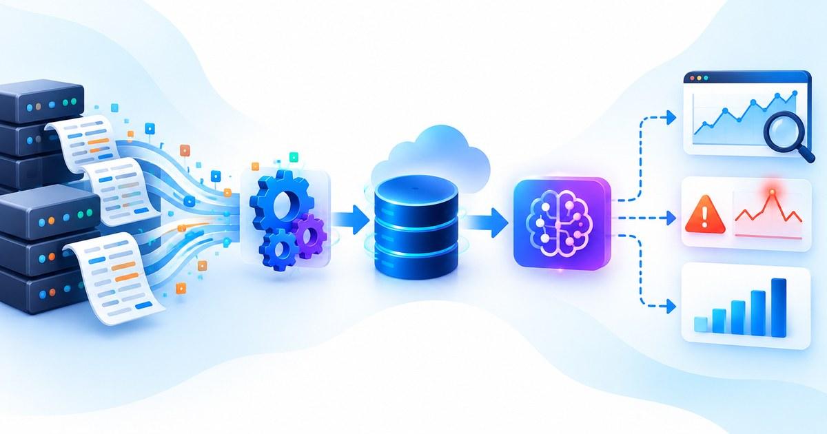
A predictive autoscaling architecture connects workload telemetry, machine learning forecasts, and infrastructure control mechanisms so that future resource requirements can influence scaling decisions before demand increases. The system typically begins with an observability pipeline that collects metrics from application services, containers, cloud resources, and request-processing queues, after which a forecasting component analyzes historical and recent observations to estimate demand over a defined future time window. A scaling controller then translates these estimates into operational actions, taking into account currently available capacity, provisioning delays, resource limits, and the performance objectives of the application rather than allowing a forecasting model to modify infrastructure without defined constraints.
Separating forecasting from infrastructure control is important because the two components solve different problems and require different validation strategies. The forecasting service estimates future workload characteristics, such as incoming request volume or expected CPU consumption, while the controller determines whether additional replicas or compute resources are needed to satisfy the application's requirements. For example, a forecast predicting a substantial increase in API traffic does not automatically imply that the deployment should double its replica count, since the appropriate adjustment depends on the throughput of each instance, current capacity, latency objectives, and the amount of uncertainty associated with the prediction.
This architecture also benefits from treating forecast outputs as versioned, time-sensitive data with explicit timestamps, prediction horizons, and confidence estimates where available. The controller can reject stale forecasts, apply conservative capacity margins when uncertainty is high, and fall back to reactive scaling when the prediction service becomes unavailable. By maintaining this separation between prediction and actuation, engineers can update forecasting models independently from infrastructure policies while preserving predictable control behavior and limiting the consequences of inaccurate model outputs.
Combining Predictive Scaling With Reactive Autoscaling Policies
Predictive autoscaling is generally most effective when it complements conventional autoscaling mechanisms rather than replacing them, because historical patterns can anticipate recurring demand but cannot guarantee accurate predictions for every unexpected event. A reactive controller observes current metrics and responds when resource pressure or workload indicators cross configured thresholds, whereas a predictive component can initiate scale-out actions earlier when forecasts indicate that additional capacity will soon be required. Combining these mechanisms allows infrastructure to prepare for expected demand while retaining the ability to respond to traffic surges that exceed the forecast or develop too quickly for advance provisioning.
In Kubernetes environments, the Horizontal Pod Autoscaler can adjust workload replicas using observed resource metrics or supported custom and external metrics, making it useful for responding to current application conditions. Predictive scaling generally requires an additional mechanism that generates future-demand signals and translates them into scaling decisions, such as a forecasting service connected to a custom controller or an integration that exposes suitable metrics to the existing scaling workflow. Engineers must design this integration carefully to avoid competing controllers repeatedly changing replica counts, particularly when a predictive policy requests additional capacity while a reactive policy simultaneously attempts to scale the deployment in a different direction.
Coordination policies should therefore define how predictive recommendations interact with reactive thresholds, minimum and maximum replica counts, stabilization windows, and scale-in restrictions. When demand is expected to increase, the system can provision capacity in advance, while a reactive policy handles any additional pressure that emerges after traffic arrives; during periods of declining demand, gradual scale-in helps prevent premature removal of resources that remain necessary for incoming requests. These safeguards are especially valuable in latency-sensitive environments, where maintaining sufficient capacity may matter more than eliminating every instance of temporary overprovisioning, an engineering trade-off closely related to the principles in “ML for Real-Time Systems: Engineering Models Under Strict Latency Constraints.”
Translating Forecasts Into CPU, Memory, Replica, and Compute Capacity
A practical predictive autoscaling system must convert model predictions into resource decisions that reflect how an application actually consumes infrastructure, because forecasting traffic alone does not determine the amount of capacity required to serve it safely. If a forecasting model predicts the number of incoming requests over the next several minutes, the scaling controller must also estimate how much processing capacity each replica can sustain while meeting the required latency and error-rate objectives. This translation can use measured throughput, observed resource consumption, historical performance tests, and a configurable safety margin, allowing the system to determine whether additional replicas, larger instances, or different compute resources would best accommodate the anticipated workload.
Resource planning becomes more complex when CPU, memory, and concurrency constraints interact, since increasing the number of replicas may not resolve bottlenecks in shared databases, external APIs, storage systems, or other constrained dependencies. A request-heavy application might benefit from additional application replicas, but scaling those replicas without accounting for database connection limits could increase contention and worsen response times. Predictive autoscaling should therefore consider relevant dependency metrics and downstream capacity constraints, ensuring that a forecast-driven scale-out action does not simply transfer the bottleneck to another part of the system.
The forecasting horizon must also reflect the time required to bring usable capacity online, since an accurate prediction delivered too late may provide little practical benefit. If a workload requires several minutes to provision and initialize new instances, the system needs a forecast that reaches far enough into the future to accommodate that delay, while retaining shorter-horizon predictions or reactive controls for rapidly developing demand changes. Engineers can calibrate the scaling policy by comparing predicted requirements with actual resource consumption across different workload conditions, gradually improving its capacity estimates without allowing experimental forecasting logic to bypass established infrastructure limits.
Key Takeaway
A predictive autoscaling architecture connects historical telemetry and machine learning forecasts to a controlled infrastructure scaling mechanism, enabling cloud and Kubernetes workloads to prepare for expected demand before resource pressure becomes critical. Reliable implementations separate forecasting from infrastructure control, combine proactive decisions with reactive autoscaling, translate demand estimates into realistic capacity requirements, and enforce safeguards against forecast errors, scaling oscillations, and resource constraints. This combination enables engineering teams to anticipate predictable workload changes while retaining the operational resilience required to handle unexpected traffic and infrastructure limitations.
Section 4: Operating Predictive Autoscaling in Production: Reliability, Cost, and Performance
Measuring the Impact of Predictive Scaling on Latency and Availability
Operating predictive autoscaling in production requires engineers to measure whether anticipating infrastructure demand actually improves application performance, rather than assuming that more accurate forecasts automatically produce better operational outcomes. A forecasting model may estimate upcoming traffic with reasonable accuracy, yet the scaling policy can still perform poorly if it provisions capacity too late, allocates resources inefficiently, or overlooks bottlenecks in downstream dependencies. Teams should therefore evaluate the complete scaling workflow using metrics such as average and tail latency, request error rates, availability, resource utilization, provisioning time, and the frequency of capacity-related incidents, comparing these measurements against a suitable reactive autoscaling baseline under comparable workload conditions.
Latency percentiles are particularly important because averages can conceal the performance degradation experienced by a relatively small proportion of users during demand spikes. For example, predictive scaling may improve average response times while leaving p99 latency elevated because database connections remain saturated or newly provisioned instances require substantial initialization before becoming effective. Measuring performance across different traffic levels helps engineers identify whether the additional capacity is arriving early enough to protect service-level objectives, while correlating latency with queue depth, instance readiness, and resource consumption provides evidence about where further optimization is necessary.
Availability and reliability measurements should also account for the consequences of unexpected forecast errors, since a system that performs well during predictable daily peaks may still struggle when demand changes abruptly. Controlled load tests, historical workload replay, and staged production experiments can reveal how the scaling strategy responds to both recurring traffic patterns and sudden surges, allowing teams to refine forecasting horizons, capacity margins, and fallback policies before relying heavily on predictive decisions.
Preventing Overprovisioning and Measuring Infrastructure Cost Savings
Although predictive autoscaling can reduce the need to maintain excessive standby capacity, inaccurate forecasts can introduce new forms of infrastructure waste when the system provisions resources for demand that never materializes. If a forecasting model consistently overestimates upcoming traffic, cloud instances may remain underutilized throughout the period for which they were provisioned, increasing compute expenditure without producing meaningful performance improvements. Engineers must therefore evaluate capacity utilization alongside application responsiveness, considering whether forecast-driven scaling reduces the combined cost of idle resources and performance degradation rather than optimizing either metric in isolation.
Cost measurement should include the full infrastructure footprint associated with predictive autoscaling, including the monitoring pipeline, forecasting service, model inference, additional storage, orchestration components, and any temporary capacity provisioned ahead of expected demand. For relatively simple workloads, a lightweight statistical forecast or scheduled scaling rule may produce most of the operational benefit at a lower cost than a more sophisticated ML model, making the complexity of the forecasting approach an important part of the economic evaluation. Teams can assess the business case by measuring infrastructure expenditure per request, resource utilization during peak and off-peak periods, the duration of unused capacity, and the cost of incidents associated with insufficient provisioning.
The principles discussed in “The Economics of Machine Learning: Measuring the True Cost of a Model” are useful when evaluating whether the predictive component delivers sufficient value to justify its ongoing operational expense, particularly when the forecast itself consumes resources or requires regular maintenance. By comparing predictive scaling against simpler alternatives and measuring results over representative workload cycles, engineering teams can establish whether the architecture creates measurable savings while preserving the latency and availability requirements of the application.
Monitoring Forecast Drift and Adapting to Changing Workloads
Predictive autoscaling systems must continuously evaluate forecast quality because the relationships between historical metrics and future demand can change as applications evolve, user behavior shifts, or new features alter resource consumption. A forecasting model trained on several months of relatively stable traffic may become less reliable after a major product launch or a change in the distribution of incoming requests, particularly when these changes affect the amount of compute required for each request. Monitoring forecast residuals, which represent the differences between predicted and observed demand, helps engineers identify systematic underestimation or overestimation before those errors repeatedly influence infrastructure decisions.
Forecast evaluation should consider both aggregate accuracy and performance during operationally significant periods, since a model may appear accurate across an entire week while consistently underpredicting the busiest intervals. Teams can track prediction errors across different forecast horizons, traffic levels, and workload categories, comparing them against predefined tolerances to determine when a forecasting model requires investigation or adjustment. Because actual demand measurements become available only after the corresponding prediction period has passed, the monitoring architecture must preserve timestamped forecasts and observed metrics so that errors can be calculated consistently and associated with the model version responsible for each prediction.
Model retraining may improve performance when workload patterns have changed sufficiently, but automatic retraining should not immediately translate into uncontrolled production changes without evaluation against representative data. A safer process validates candidate models against recent workloads, compares their forecast performance with the current model, and introduces updates through controlled deployment procedures while retaining a known-good alternative. This approach helps the infrastructure adapt as demand evolves without assuming that every observed deviation represents permanent drift or that a newly trained model will necessarily perform better under future conditions.
Key Takeaway
Operating predictive autoscaling successfully requires continuous measurement of application performance, infrastructure expenditure, forecast reliability, and the safety of scaling decisions. By comparing results against reactive baselines, monitoring forecast errors across changing workloads, deploying improvements gradually, and preserving reactive fallback mechanisms, engineering teams can anticipate infrastructure demand while controlling operational risk and avoiding unnecessary provisioning. The objective is not simply to predict future traffic accurately, but to use those predictions to deliver measurable improvements in availability, responsiveness, and infrastructure efficiency.
Conclusion: Moving From Reactive Scaling to Predictive Infrastructure Management
Predictive autoscaling represents an important evolution in cloud infrastructure management by enabling engineering teams to anticipate resource requirements instead of relying exclusively on reactive responses to rising utilization. Traditional autoscaling remains effective for handling immediate changes in workload conditions, but its dependence on current metrics can introduce delays while additional capacity is provisioned, initialized, and prepared to serve traffic. By applying machine learning to historical telemetry, workload patterns, and recent operational signals, predictive autoscaling can estimate upcoming demand and initiate capacity adjustments early enough to improve responsiveness, reduce performance degradation, and make more efficient use of infrastructure resources.
Building an effective predictive autoscaling system requires more than selecting a forecasting algorithm because the complete architecture must connect reliable telemetry collection, workload prediction, capacity estimation, infrastructure orchestration, and operational monitoring. Statistical forecasting methods and machine learning models can identify recurring traffic patterns and estimate future resource requirements, while a dedicated scaling controller translates those predictions into bounded infrastructure actions that account for provisioning delays, service-level objectives, resource quotas, and the capacity already available. This separation allows engineering teams to improve forecasting independently from infrastructure control, making the system easier to evaluate, maintain, and adapt as application requirements evolve.
Production reliability depends on combining predictive scaling with reactive safeguards rather than assuming that future demand can always be forecast accurately. Unexpected traffic surges, changing user behavior, deployment-related workload changes, and infrastructure constraints can all cause actual demand to diverge from model predictions, making real-time monitoring, controlled scaling actions, and fallback policies essential components of the design. Engineers must also evaluate the quality of the resulting infrastructure decisions by monitoring latency percentiles, availability, resource utilization, forecast errors, provisioning delays, and total operating costs, ensuring that improved prediction accuracy translates into measurable operational benefits.
The economic value of predictive autoscaling ultimately depends on whether the system provides sufficient performance and reliability improvements to justify its implementation and maintenance costs. For some applications, scheduled scaling or a well-configured reactive autoscaler may already handle workload variation efficiently, while services with recurring traffic peaks, expensive compute resources, or long initialization times may benefit substantially from proactive capacity planning. A practical implementation should therefore begin with a measurable infrastructure problem, establish a reactive baseline, validate forecasts against historical workloads, and introduce predictive controls gradually while preserving established safety mechanisms.
By treating machine learning as a decision-support component within a carefully designed infrastructure control system, software and platform engineers can move toward more proactive capacity management without surrendering operational control to imperfect predictions. The strongest predictive autoscaling architectures combine reliable forecasting, workload-aware capacity planning, reactive recovery mechanisms, and continuous performance evaluation to deliver infrastructure that responds intelligently to changing demand while balancing application responsiveness, availability, and cloud expenditure.
Frequently Asked Questions
1. What Is Predictive Autoscaling?
Predictive autoscaling is an infrastructure management technique that forecasts future workload demand and adjusts computing capacity before the anticipated demand arrives. It uses historical metrics, recent workload observations, and forecasting algorithms to estimate upcoming resource requirements, allowing cloud applications to prepare additional capacity in advance rather than waiting for current utilization to exceed a configured threshold.
2. How Is Predictive Autoscaling Different From Reactive Autoscaling?
Reactive autoscaling adjusts infrastructure in response to observed conditions, such as elevated CPU utilization, increasing request volume, or growing message queues, whereas predictive autoscaling uses forecasts to anticipate future conditions before they occur. Predictive scaling can reduce delays associated with resource provisioning and initialization, while reactive scaling remains essential for handling unexpected traffic spikes, forecast errors, and workload changes that develop too quickly for advance preparation.
3. How Does Machine Learning Help Predict Infrastructure Demand?
Machine learning helps forecast infrastructure demand by identifying patterns and relationships in historical telemetry, including request rates, resource consumption, traffic seasonality, queue growth, and workload characteristics. Depending on the application, models can estimate future request volume, CPU utilization, memory requirements, or capacity needs, providing infrastructure controllers with information that supports earlier and more informed scaling decisions.
4. Which Machine Learning Models Are Suitable for Predictive Autoscaling?
The appropriate model depends on workload complexity, data availability, forecast horizon, and operational requirements, with statistical methods such as autoregressive integrated moving average models and exponential smoothing providing useful baselines for recurring time-series patterns. Tree-based models, including gradient-boosted decision trees, can incorporate multiple operational signals, while neural networks designed for sequential data may help capture more complex temporal relationships when the available data supports their additional complexity.
5. What Metrics Are Required to Implement Predictive Autoscaling?
A predictive autoscaling system typically benefits from historical CPU and memory utilization, request rates, concurrent requests, response latency, queue depth, replica counts, and resource provisioning times. Depending on the workload, engineers may also incorporate calendar features, scheduled jobs, deployment events, cache behavior, and relevant business activity, provided that the collected data is consistent, sufficiently detailed, and representative of the operating conditions the model must forecast.
6. Can Predictive Autoscaling Be Implemented in Kubernetes?
Yes, predictive autoscaling can be implemented in Kubernetes by connecting a forecasting component to a scaling controller that can adjust workload capacity according to predicted demand. Kubernetes Horizontal Pod Autoscaler supports scaling based on observed resource metrics and supported custom or external metrics, while predictive capabilities generally require an additional forecasting mechanism or integration that translates future-demand estimates into appropriate scaling signals or replica adjustments.
7. Should Predictive Autoscaling Replace the Kubernetes Horizontal Pod Autoscaler?
Predictive autoscaling should generally complement rather than replace reactive scaling mechanisms because forecasts can prepare infrastructure for expected workloads but cannot anticipate every unexpected event. A combined architecture can scale out proactively when forecast demand increases, use reactive policies to respond to additional resource pressure, and apply stabilization rules to prevent premature scale-in or conflicting scaling actions.
8. How Far Ahead Should an Autoscaling System Forecast Demand?
The forecasting horizon should reflect how quickly workload demand changes and how long the infrastructure takes to provision, initialize, and become ready to serve traffic. Applications with rapid container startup times may need relatively short forecasting horizons, whereas workloads involving large model artifacts, specialized compute resources, or lengthy initialization procedures may require earlier predictions, with the chosen horizon validated against historical workload patterns and measured provisioning delays.
9. How Accurate Must a Predictive Autoscaling Model Be?
The required forecasting accuracy depends on the consequences of underestimating or overestimating demand, the cost of maintaining spare capacity, and the time required to provision additional resources. Instead of relying on one universal accuracy threshold, engineers should evaluate prediction errors across multiple forecast horizons and workload conditions, paying particular attention to peak-demand underestimation, provisioning readiness, service-level objectives, and the actual operational outcomes produced by the scaling policy.
10. How Does Predictive Autoscaling Reduce Cloud Infrastructure Costs?
Predictive autoscaling can reduce infrastructure costs by provisioning capacity when demand is expected to rise and removing excess resources when demand declines, helping applications avoid both insufficient capacity and unnecessarily large standby fleets. However, savings are not guaranteed because inaccurate forecasts, excessive safety margins, forecasting infrastructure, and inefficient scaling policies can introduce additional expenditure, making comparisons against a well-configured reactive baseline essential for determining the financial value of the implementation.
11. What Are the Main Challenges of Predictive Autoscaling?
The principal challenges include collecting reliable historical telemetry, selecting appropriate forecasting models, accounting for infrastructure startup delays, translating predicted demand into capacity requirements, and handling workload changes that differ from historical patterns. Engineering teams must also prevent scaling oscillations, avoid overprovisioning, coordinate predictive and reactive controllers, and preserve safe behavior when forecasts become stale or infrastructure resources cannot be provisioned as expected.
12. How Can Predictive Autoscaling Handle Unexpected Traffic Spikes?
Predictive autoscaling can handle unexpected traffic spikes most effectively when it is combined with reactive monitoring and scaling policies that respond to actual workload conditions. If incoming requests exceed the forecast, real-time signals such as rising CPU utilization, increasing concurrency, elevated latency, or rapidly growing queues can trigger additional scaling actions, while preconfigured capacity limits and fallback policies help maintain control during unusually severe demand changes.
13. How Can Engineers Prevent Overprovisioning With Predictive Autoscaling?
Overprovisioning can be reduced by evaluating historical forecast errors, incorporating realistic capacity estimates, limiting scaling actions, and continuously comparing predicted resource requirements with actual utilization. Teams should also establish suitable minimum and maximum capacity bounds, apply stabilization windows where appropriate, and measure the costs of unused resources alongside the performance consequences of insufficient capacity, allowing scaling policies to balance application reliability with infrastructure expenditure.
14. How Should Predictive Autoscaling Be Monitored in Production?
Production monitoring should cover both forecasting quality and infrastructure outcomes, including prediction errors, latency percentiles, request failures, replica availability, provisioning delays, resource utilization, and total operating costs. By recording timestamped predictions and comparing them with subsequent observations, engineering teams can identify systematic forecasting errors, detect changing workload behavior, assess whether scaling actions improve service performance, and determine when a model or scaling policy requires adjustment.
15. When Should an Engineering Team Adopt Predictive Autoscaling?
Predictive autoscaling is especially worth evaluating when an application experiences recurring demand peaks, long infrastructure startup times, strict latency requirements, expensive compute capacity, or significant resource waste caused by conservative provisioning. Teams should first determine whether scheduled scaling or conventional reactive autoscaling already meets their requirements, then validate predictive approaches against historical workloads and measurable operational objectives before introducing production controls, ensuring that the resulting benefits justify the complexity of maintaining the forecasting system.