Shadow Deployment for ML Models: Testing New Predictions Without Affecting Users

Section 1: Understanding Shadow Deployment and Its Role in Production ML

What Is Shadow Deployment in Machine Learning?

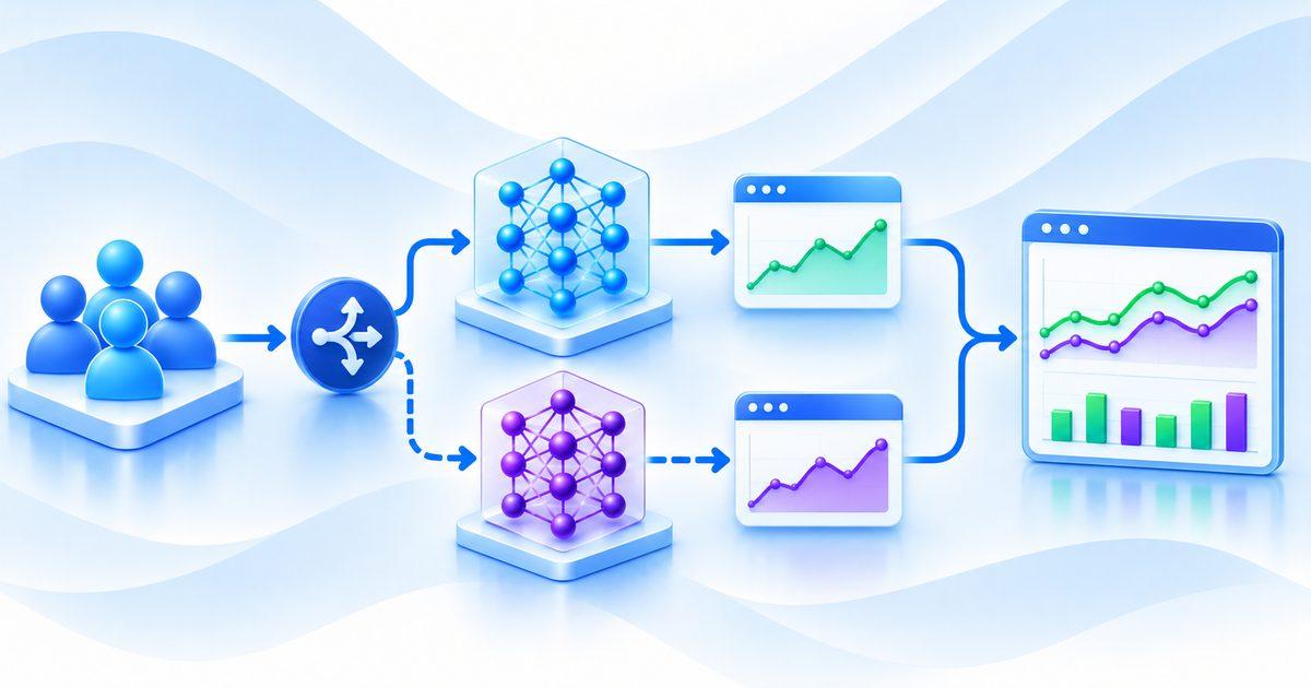
Shadow deployment is a production testing strategy that allows machine learning engineers to evaluate a new model using real production inputs without allowing its predictions to influence user-facing decisions. The existing production model continues handling requests and generating the predictions used by the application, while a candidate model receives copies of those same requests and processes them independently. This parallel execution allows teams to observe how the candidate behaves under actual production conditions before deciding whether it is suitable for a controlled rollout.

The existing model is commonly referred to as the champion, while the candidate being evaluated is called the challenger. For example, an e-commerce company may operate a recommendation model that ranks products based on customer activity, purchase history, and contextual features. When engineers develop a new recommendation model, they can mirror incoming customer requests to both versions, allowing the champion to return recommendations to users while the challenger generates alternative rankings that are recorded for later analysis. Customers continue receiving recommendations from the existing system, but the engineering team gains evidence about how the new model behaves when exposed to genuine traffic.

The defining characteristic of shadow deployment is the separation between prediction generation and application decision-making. The candidate model can calculate scores, probabilities, rankings, or classifications, but those outputs must not trigger transactions, update customer records, generate notifications, or influence the response returned to the user. This separation makes shadow deployment particularly useful when replacing models in systems where incorrect predictions could affect financial transactions, fraud investigations, search results, healthcare workflows, or customer experiences. It also allows engineers to identify operational problems, such as excessive inference latency, unexpected input formats, or resource consumption, before exposing users to the candidate model.

Why Offline Model Evaluation Is Not Enough

Offline evaluation is an essential part of machine learning development because it allows engineers to compare models using historical datasets, measure predictive performance, and identify weaknesses before deployment. However, historical test data cannot reproduce every condition that a model will encounter in a live application, where user behavior, traffic volume, feature availability, and operational constraints may differ from the development environment. A model that performs well on a carefully prepared validation dataset may therefore produce unexpected predictions or experience infrastructure problems when it processes actual production requests.

Consider a fraud detection model trained using historical transaction records, where offline evaluation demonstrates strong precision and recall across the test dataset. After deployment, the model may encounter new transaction patterns, unusual combinations of features, delayed customer information, or a sudden increase in request volume that were not adequately represented during development. Its predictive behavior may differ from the offline results, while the serving infrastructure may also experience higher latency or resource consumption than expected. These problems cannot always be identified through another round of testing against the same historical dataset because the underlying conditions remain unchanged.

The gap between offline evaluation and production behavior is closely related to differences in training data, serving features, and the environment in which predictions are generated. Production features may be missing, delayed, or calculated using different aggregation windows, while changing user behavior can introduce input distributions that were uncommon during training. As explained in “Why Machine Learning Models Behave Differently in the Real World”, strong offline metrics do not guarantee production performance because real applications introduce changing data, operational constraints, and user interactions that historical evaluation cannot fully reproduce. Shadow deployment addresses part of this validation gap by allowing a candidate model to process live inputs without making it responsible for production decisions.

How Shadow Deployment Works: Production Model and Challenger Model

A typical shadow deployment architecture begins when an application receives a request and sends it through the normal production serving path. The serving infrastructure forwards the request to the existing model and creates a separate copy for the candidate model, ensuring that both versions receive equivalent inputs whenever their feature and preprocessing requirements are compatible. The production model generates the prediction used by the application, while the candidate model processes the mirrored request independently and sends its output to a dedicated logging or evaluation system.

For example, in a search-ranking application, a customer submits a query and the production model ranks the available results before returning them to the interface. A candidate ranking model receives a copy of the same query and relevant request features, calculates its own ranking, and records the result without changing the search results displayed to the customer. Engineers can later compare ranking differences, prediction latency, error rates, and resource consumption to understand whether the challenger offers improvements or introduces new operational concerns.

Shadow inference can be implemented synchronously or asynchronously, depending on the system architecture and testing requirements. In synchronous execution, the application or serving layer may wait for both model requests to complete, although the candidate response is still excluded from the user-facing result. Asynchronous execution allows the production response to return independently while the candidate model processes the copied request through a background worker, queue, or separate inference service. This approach is generally preferable when protecting production latency is a priority because delays or failures in the candidate model do not need to hold up the primary response path.

Reliable comparison also requires request correlation and model-version tracking, since predictions must be associated with the same input and the exact model versions that generated them. Teams can use correlation IDs, timestamps, feature snapshots, model identifiers, and structured prediction logs to connect production and shadow outputs during analysis. They should also capture execution metadata, including inference duration and error status, because prediction comparison alone does not reveal whether the candidate can meet production reliability requirements. These mechanisms make shadow deployment an observable testing workflow rather than simply running two models simultaneously.

Key Takeaway

Shadow deployment allows machine learning engineers to test a candidate model against real production inputs while keeping the existing model responsible for all user-facing predictions and business decisions. By separating candidate inference from application behavior, teams can evaluate prediction differences, operational performance, and compatibility with live traffic without intentionally exposing users to unvalidated model outputs. Its greatest value comes when production conditions may reveal problems that offline evaluation cannot reproduce, making shadow testing an important validation stage before canary deployment or full production rollout.

Section 2: Designing the Architecture for Shadow Model Deployment

Traffic Mirroring and Request Duplication Architecture

A shadow deployment architecture begins with the ability to duplicate production requests and route them to a candidate model without changing the normal application response path. When an application receives a request, the existing inference service processes it as usual, while a separate component creates a copy that is delivered to the shadow model. This duplication can happen at an API gateway, load balancer, application service, message broker, or dedicated inference gateway, depending on the system's architecture and where the required model inputs are available. The objective is to ensure that both models evaluate equivalent production inputs while keeping the candidate's execution independent of the primary serving workflow.

The location of traffic duplication influences the consistency and complexity of the architecture. Mirroring at the API gateway can capture incoming requests before they enter application-specific processing, but the duplicated payload may not contain all the features required by the model. Duplicating traffic at the application or inference layer can provide access to enriched request data, including calculated features, user context, and preprocessing outputs, making it easier to reproduce the inputs used by the production model. Engineers should therefore identify the exact point at which the model receives its final feature representation and determine whether the candidate requires the same representation or a separately versioned transformation.

Request duplication must preserve the information needed for reliable comparison without unnecessarily increasing data exposure or processing overhead. Correlation IDs, request timestamps, model version identifiers, feature schema versions, and relevant request metadata help associate candidate predictions with their corresponding production predictions. When candidate and production models use different feature schemas, engineers should explicitly map or transform the inputs rather than assuming that identical raw requests will produce equivalent model inputs. Traffic sampling can also reduce the volume of shadow requests when processing every production request would consume excessive compute resources, provided that the selected sample remains representative of the traffic patterns being evaluated.

Synchronous Versus Asynchronous Shadow Inference

Synchronous shadow inference executes the production and candidate model requests within the same request-handling workflow, allowing both predictions to be generated from the same incoming request before the workflow completes. Although the candidate output remains excluded from the user-facing response, waiting for the candidate to finish can increase end-to-end latency and make the primary application more sensitive to shadow-model delays. This approach may be appropriate in controlled environments where predictable execution and immediate prediction comparison are important, but it requires careful timeout handling and strict separation of model failures from application responses.

Asynchronous shadow inference avoids making the primary response dependent on the candidate model's execution time by returning the production prediction while submitting the copied request to a background processing path. The duplicated request can be published to a message queue or event stream, where independent workers retrieve it and invoke the candidate inference service. This design is generally preferable for latency-sensitive applications because a slow candidate model does not need to delay the user's request, while failures in the shadow processing pipeline can be recorded and investigated without interrupting normal application behavior. For example, an e-commerce application can return search results from its existing ranking model while a background worker evaluates the same search request using a new ranking model.

Asynchronous processing introduces its own operational requirements because queues, workers, and inference services must handle variable request volumes without creating an uncontrolled backlog. Engineers should configure bounded queues, processing limits, timeouts, retry policies, and backpressure mechanisms so that shadow workloads do not consume unlimited memory or overwhelm downstream services during traffic spikes. They should also define how duplicate messages, delayed execution, and failed candidate requests are handled, particularly when the comparison process depends on associating predictions with the original production request. These controls allow teams to preserve the independence of the shadow workflow while maintaining visibility into how much production traffic is actually being evaluated.

Isolating Shadow Predictions From Production Decisions and Side Effects

Separating candidate predictions from business decisions is one of the most important architectural requirements of shadow deployment because the candidate model is being evaluated, not trusted to control application behavior. Its outputs should be directed to an isolated prediction store, evaluation service, or dedicated logging pipeline rather than being passed into the normal decision-making components. A candidate fraud detection model, for example, may generate a high-risk score for a transaction, but that score must not block the payment, trigger a fraud investigation, or update the customer's account while the model remains in shadow mode. The incumbent model should continue to determine the actual production outcome until the candidate has passed the required evaluation and has been approved for a controlled release.

This separation must extend beyond the model endpoint because downstream application services may interpret any prediction as an instruction to perform an action. If a shadow recommendation model writes its rankings into the live recommendation database, or a candidate fraud model triggers the same notification workflow as the production model, the deployment is no longer safely isolated even if the application response still comes from the incumbent model. Engineers should therefore use read-only access wherever possible, dedicated credentials, independent output destinations, and explicit controls that prevent shadow execution from invoking transaction processing or other side-effecting operations. Testing should also verify that candidate requests cannot accidentally reach production write endpoints through shared service logic or incorrectly configured integrations.

The integration principles discussed in “Building ML Features Into Existing Applications: A Step-by-Step Engineering Approach” are relevant because shadow inference must coexist with existing application services without allowing model-specific behavior to disrupt established workflows. Engineers should maintain clear service boundaries, define stable request and response contracts, and distinguish between prediction generation and the business logic that consumes predictions. This separation makes it easier to test candidate models independently, investigate unexpected outputs, and promote a model later without introducing hidden dependencies between its inference implementation and the application's existing transaction or decision pathways.

Key Takeaway

A reliable shadow deployment architecture requires controlled traffic duplication, appropriate synchronous or asynchronous execution, strict isolation of candidate outputs, and sufficient infrastructure capacity to process mirrored requests without disrupting the primary serving path. Engineers should preserve request consistency through correlation and version tracking, use queues and backpressure when asynchronous processing is required, and ensure that candidate predictions cannot trigger real business actions or production data changes. Resource monitoring, workload isolation, and privacy-aware data handling complete the architecture, allowing teams to test new models under realistic production conditions while preserving the stability and security of the existing application.

Section 3: Comparing Model Predictions and Evaluating Shadow Performance

Comparing Predictions Between the Production and Shadow Models

One of the primary objectives of shadow deployment is to understand how a candidate model behaves when it receives the same production inputs as the existing model. Since both models process equivalent requests, engineers can compare their predictions to identify differences in classification outcomes, probability estimates, numerical forecasts, or ranking decisions. This comparison provides an early indication of how the candidate might change application behavior if it were promoted, although prediction agreement alone cannot establish which model is more accurate or whether the candidate delivers greater business value.

The comparison approach depends on the type of machine learning problem being evaluated. For a classification model, engineers can compare predicted classes, probability distributions, confidence scores, and decision-threshold behavior to identify cases where the challenger makes a different classification from the champion. For regression systems, the comparison may involve absolute prediction differences, percentage deviations, and changes in predicted values across different input ranges, while recommendation and search-ranking systems require examining changes in item rankings, relevance scores, and the positions assigned to important results. A fraud detection model, for example, may classify a transaction as low risk while the candidate assigns it a substantially higher risk score, making the disagreement a useful signal for further investigation.

Prediction differences should be analyzed across relevant segments rather than being reduced to a single aggregate disagreement rate. A candidate model may produce results similar to the existing model for most customers but behave differently for new users, high-value transactions, specific geographical regions, or uncommon input combinations. Engineers can group disagreements by feature ranges, customer categories, request types, and other relevant dimensions to identify patterns that might indicate changes in model behavior or feature compatibility. They should also distinguish expected differences caused by a new model design from unexpected changes caused by missing features, preprocessing inconsistencies, or incorrect request transformations, since these problems require different corrective actions.

Measuring Prediction Quality When Ground-Truth Labels Are Delayed

A major challenge in shadow deployment is that production ground-truth labels are not always available when predictions are generated. Some machine learning applications receive feedback immediately, but others require time before the actual outcome can be established reliably. In fraud detection, a transaction may be identified as fraudulent only after an investigation, while customer churn may become observable several weeks after a prediction indicates that a customer is likely to discontinue a service. Similarly, recommendation systems may require subsequent user interactions before engineers can determine whether a ranking generated meaningful engagement or contributed to a purchase.

When labels are delayed, engineers should preserve sufficient prediction metadata to connect future outcomes with the model outputs that were generated earlier. Each recorded prediction should contain information such as the request identifier, timestamp, model version, prediction value, relevant feature version, and evaluation context, subject to appropriate privacy and retention controls. Once the corresponding outcome becomes available, the evaluation pipeline can associate it with the original prediction and calculate model quality metrics using the correct version of the model. This temporal association is particularly important when several candidate models are evaluated simultaneously or when the production model changes during the observation period.

During the waiting period, teams can monitor operational behavior and carefully selected proxy indicators without treating them as substitutes for actual predictive accuracy. For example, a recommendation model may be evaluated initially through ranking stability, inference latency, and the distribution of recommended products, while click-through rate and conversion outcomes require sufficient subsequent user activity. A fraud detection model may be assessed for risk-score distributions and processing reliability before confirmed fraud labels become available, although these observations cannot establish whether the candidate is correctly identifying fraudulent transactions. Separating immediate operational evidence from delayed predictive evaluation prevents teams from promoting a model based on misleading early indicators.

Establishing Acceptance Criteria for Promoting a Shadow Model

Before beginning a shadow evaluation, engineering teams should define measurable acceptance criteria that determine whether the candidate model is ready for the next deployment stage. These criteria should combine predictive evidence, operational reliability, infrastructure requirements, and application-specific business objectives rather than relying on a single measure of agreement with the existing model. For example, a candidate fraud detection model may need to demonstrate acceptable recall and precision once confirmed labels become available, maintain inference latency within the service's established limits, and avoid unexpected prediction changes across important transaction categories. A recommendation model may instead require evidence of ranking quality, acceptable resource consumption, and no significant deterioration in relevant customer segments.

Acceptance criteria should also specify the required observation period and the amount of production traffic needed to make the evaluation meaningful. A short testing window may fail to capture weekly behavior, seasonal patterns, traffic spikes, or rare input conditions, while an extremely small traffic sample may not provide enough evidence about less common scenarios. Teams should select an observation period based on the application's traffic patterns, label availability, risk level, and expected data variability, while documenting cases that remain insufficiently evaluated. They should also distinguish hard operational requirements, such as maximum allowable latency or error rates, from predictive objectives that require statistical interpretation and sufficient ground-truth evidence.

The final decision should be based on predefined evidence showing whether the candidate is ready for promotion, requires additional optimization, or should be rejected. Engineers should investigate unexpected prediction disagreements, examine performance across relevant segments, verify feature compatibility, and assess whether the candidate can operate within production resource constraints before allowing it to influence live decisions. The testing principles discussed in “ML Testing for Software Engineers: How to Test Systems That Don't Always Produce the Same Output” are relevant because evaluating machine learning systems requires behavioral comparisons, statistical measurements, and operational validation rather than relying exclusively on deterministic pass-or-fail checks. Once the candidate satisfies the agreed criteria, teams can use the results as evidence for a controlled canary deployment, where its predictions begin influencing a limited portion of real application traffic under continued monitoring.

Key Takeaway

Evaluating a shadow model requires more than comparing its predictions with those of the existing production model, because agreement does not establish correctness and differences do not automatically indicate improvement. Engineering teams should combine prediction comparison, delayed ground-truth evaluation, feature and output distribution monitoring, latency measurements, and infrastructure observability to understand how the candidate behaves under realistic production conditions. By defining acceptance criteria before testing begins and using measurable evidence to guide promotion decisions, teams can determine whether a candidate is ready for a controlled rollout without exposing users to unvalidated predictions.

Conclusion: Making Shadow Deployment a Standard Practice in Production ML

Deploying a new machine learning model into a production environment involves more than achieving strong validation metrics or demonstrating improvements on historical datasets, because real-world applications introduce changing traffic patterns, unexpected input combinations, infrastructure constraints, and operational dependencies that cannot always be reproduced offline. Shadow deployment addresses part of this challenge by allowing a candidate model to process actual production requests while the existing model continues generating the predictions used by the application. This approach gives engineering teams an opportunity to observe candidate behavior under realistic conditions without intentionally exposing users to unvalidated predictions or allowing the candidate to influence business decisions.

The effectiveness of shadow deployment depends on designing a reliable architecture that separates request duplication, candidate inference, and prediction evaluation from the primary application response path. Traffic mirroring allows both models to process equivalent inputs, while asynchronous inference, independent processing queues, resource isolation, and dedicated prediction storage help prevent candidate execution from interfering with production services. Engineers must also ensure that shadow predictions cannot trigger transactions, database modifications, notifications, or other business side effects, because even a model operating in shadow mode can introduce operational risks when its outputs are connected to live application workflows. Privacy controls and infrastructure monitoring are equally important because mirrored production requests may contain sensitive information and create additional computational demand.

For machine learning and platform engineering teams, the objective of shadow deployment is not simply to run two models simultaneously, but to reduce uncertainty before changing the behavior of a production application. Organizations that implement reliable traffic mirroring, isolate candidate predictions, monitor operational performance, and use measurable acceptance criteria can introduce model improvements with greater confidence while protecting existing user experiences. As production ML systems become increasingly connected to critical business workflows, shadow deployment offers a practical engineering discipline for validating new predictions before allowing them to influence real decisions.

Frequently Asked Questions

1. What is shadow deployment in machine learning?

Shadow deployment is a production testing strategy in which a candidate machine learning model receives copies of real production requests while the existing model continues generating the predictions used by the application. The candidate processes the inputs and produces predictions that can be recorded and evaluated, but its outputs are not used to make actual user-facing decisions. This allows engineering teams to examine model behavior under realistic production conditions before considering a controlled rollout.

2. How does shadow deployment work in a production ML system?

When an application receives a request, the serving infrastructure sends it to the existing production model and creates a duplicate for the candidate model. The production model returns its prediction through the normal application response path, while the candidate independently processes the mirrored request and sends its output to a separate logging or evaluation system. Engineers subsequently compare predictions, inference latency, errors, feature behavior, and resource consumption to determine whether the candidate is suitable for further testing.

3. What is the difference between shadow deployment and canary deployment?

Shadow deployment allows a candidate model to process production requests without using its predictions to control actual application decisions, whereas canary deployment gradually routes a controlled portion of live traffic to the candidate. In a canary release, the new model's predictions can affect the experience or outcome received by real users within the selected traffic segment. Shadow deployment is therefore primarily used to gather production evidence before exposure, while canary deployment evaluates the candidate under limited real-world decision-making conditions.

4. How is shadow deployment different from A/B testing?

Shadow deployment compares candidate predictions with the existing model's predictions while ensuring that only the existing model controls the application response. A/B testing assigns users or requests to different experiences so that the organization can compare outcomes such as conversions, engagement, retention, or transaction completion. Shadow deployment is useful for examining production compatibility and model behavior without intentionally changing user experiences, whereas A/B testing is designed to measure the impact of alternative experiences on actual outcomes.

5. Do shadow models affect predictions returned to users?

A correctly implemented shadow model should not affect the predictions or decisions returned to users because its outputs are isolated from the primary application response path. The existing production model remains responsible for generating the actual response, while the candidate's predictions are stored separately for evaluation. However, poorly isolated shadow workloads can indirectly affect users through resource contention, excessive network traffic, or shared infrastructure, making capacity planning and workload isolation essential.

6. What is traffic mirroring in machine learning?

Traffic mirroring is the process of duplicating incoming production requests and forwarding copies to another service or model for independent processing. In machine learning, it allows an existing production model and a candidate model to receive equivalent inputs so that engineers can compare their behavior under realistic conditions. Traffic can be mirrored at an API gateway, load balancer, application service, or inference gateway, depending on where the required model features become available.

7. Should shadow inference be synchronous or asynchronous?

Asynchronous shadow inference is generally preferable for production applications where protecting user-facing latency is important because the primary response can be returned without waiting for the candidate model to finish processing. The mirrored request can be sent to a message queue or background worker, allowing the candidate to execute independently while its output is recorded for later evaluation. Synchronous execution may be useful in controlled testing environments that require immediate comparison, but it introduces additional latency and requires careful timeout and failure isolation.

8. How do engineers compare predictions from production and shadow models?

Engineers compare outputs generated by the champion and challenger models using identical or appropriately aligned production inputs, examining differences according to the type of machine learning task. Classification comparisons may include predicted labels, probability distributions, and confidence scores, while regression comparisons may focus on numerical deviations and ranking systems may examine changes in item positions and relevance scores. These differences should also be analyzed across relevant customer groups, request categories, and feature ranges because aggregate agreement can conceal important behavioral changes in specific segments.

9. How can teams evaluate shadow models when ground-truth labels are delayed?

When actual outcomes are not immediately available, teams should preserve prediction metadata, including model versions, request identifiers, timestamps, and relevant feature information, so that future labels can be associated with the correct predictions. Immediate evaluation can focus on operational behavior, prediction distributions, feature compatibility, and carefully selected proxy indicators, while predictive accuracy is assessed after reliable ground-truth outcomes become available. This separation prevents engineering teams from treating early operational observations or proxy metrics as definitive evidence that a candidate model is more accurate.

10. What metrics should engineers monitor during shadow deployment?

Shadow deployment monitoring should cover predictive behavior and operational performance, including inference latency, p95 and p99 response times, throughput, timeout frequency, processing errors, queue depth, CPU utilization, GPU utilization, and memory consumption. Engineers should also examine prediction distributions, confidence scores, missing-feature frequencies, output ranges, and disagreement rates between the existing and candidate models. Monitoring these measurements separately for the production and shadow services helps identify candidate-specific problems without confusing them with failures affecting the primary serving path.

11. How does shadow deployment help detect training-serving skew and data drift?

Shadow deployment exposes candidate models to actual production inputs, allowing engineers to observe differences between the data conditions encountered during training and those present during live inference. By monitoring feature distributions, missing values, unexpected categories, prediction patterns, and preprocessing behavior, teams can identify potential training-serving inconsistencies or changes in incoming data. However, shadow deployment does not automatically detect or correct every form of data drift, so it should be combined with dedicated feature monitoring, data validation, and model-performance evaluation as appropriate.

12. What are the infrastructure costs and challenges of shadow deployment?

Running an additional model alongside the production model increases inference workload and may require extra CPU, GPU, memory, network bandwidth, and storage for mirrored requests and prediction logs. Large models and high-throughput applications can create significant resource requirements, particularly when every production request is duplicated for shadow processing. Teams can manage these costs through traffic sampling, dedicated inference services, resource quotas, autoscaling, bounded queues, and workload isolation while monitoring whether shadow execution affects the primary serving infrastructure.

13. How can teams prevent shadow models from triggering real production side effects?

Candidate predictions should be directed to isolated logging or evaluation systems rather than the business components that execute transactions, update databases, send notifications, or modify customer records. Engineers should use read-only permissions, separate service credentials, independent output destinations, and explicit controls that prevent shadow requests from invoking production write operations. They should also test the complete request workflow to identify shared application logic or downstream integrations that could accidentally treat candidate predictions as instructions for real business actions.

14. When should a shadow model be promoted to a canary deployment?

A candidate should be considered for canary deployment after it satisfies predefined requirements for predictive quality, infrastructure reliability, feature compatibility, and business-specific performance. The evaluation should include sufficient production traffic and an observation period appropriate to the application's request patterns, risk level, and availability of ground-truth labels. Once the evidence supports promotion, the team can gradually route a controlled portion of real application traffic to the candidate while maintaining continuous monitoring and the ability to restore the existing model.

15. What are the best practices for implementing shadow deployment in a production MLOps pipeline?

A reliable shadow deployment pipeline should incorporate controlled traffic mirroring, request correlation, model-version tracking, isolated candidate inference, structured prediction logging, and automated evaluation. Teams should define acceptance criteria before testing, monitor both predictive and operational behavior, protect sensitive mirrored data, and ensure that shadow workloads cannot disrupt production services or trigger business side effects. Integrating shadow testing with offline validation, canary releases, model versioning, deployment automation, and rollback procedures makes it a repeatable part of the MLOps lifecycle rather than an isolated testing activity.